It is quite common in many optimization to consider the following problem:
\[\underset{x}{\text{minimize}}~\{f(x) = g(x) + h(x)\}\]
here, \( f(x) \) can be seen as total cost function, \( g(x) \) is the standard least squares cost function and \( h(x) \) is the regularization term.
If \( f(x) \) is a smooth convex function, there are many optimization techniques in the literature but for pedagogical reasons, we will mention here two most basic ones: the Newton method and the gradient descent method.
The ultimate goal of this note is to present a method for the case \( h(x) \) is nondifferentiable: the proximal gradient method.
Newton method
Consider a smooth convex function \( f(x) \), via Taylor expansion, we have:
\[f(x) = f(x_0) + \nabla f(x_0)^T (x-x_0) + (x-x_0)^T\nabla^2 f(x_0) (x-x_0) +O((x-x_0)^3)\]
At minimum position \(x_\star\)), we have \( \nabla f(x_\star) = 0\). This leads to:
\[\nabla f(x_\star) + \nabla^2 f(x_\star) (x-x_\star) +O((x-x_\star)^2) = 0\]
From this relation, we could derive the Newton algorithm as:
- initialize at \( x_0 \)
- repeat until convergence: \( x_{k+1} = x_k - (\nabla^2 f(x_k))^{-1} \nabla f(x_k) \)
Gradient descent method
Consider a smooth convex function \( f(x) \), via Taylor expansion, we have:
The conventional formulation of gradient descent algorithm is as below:
- initialize at \( x_0 \)
- repeat until convergence: \( x_{k+1} = x_k - t_{k+1} \nabla f(x_k) \)
To create a link with the proximal gradient method, we rewrite the last step as an optimization of a quadratic function as:
\[x_{k+1} = x_k - t_{k+1} \nabla f(x_k) \Longleftrightarrow x_{k+1} = \underset{x}{\text{argmin}}~f(x_k) + \nabla f(x_k)^T (x-x_k) + \frac{1}{2 t_{k+1}} ||x-x_k||^2\]
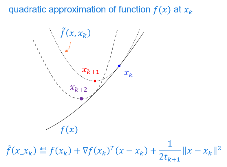
This new formulation has a nice geometric interpretation as in the below figure:

At position \(x_k\), search for a quadratic function \( \tilde{f}(x,x_k) \) so that \( \tilde{f}(x,x_k) \geq f(x) \) at the vicinity of \( x_k \), the optimization over \( f(x) \) is replaced by \( \tilde{f}(x,x_k) \). The value of \( f(x)\) at position \(x_{k+1}\) that minimizes \( \tilde{f}(x,x_k) \) should be smaller than \(f(x_k)\) since \( \tilde{f}(x,x_k) = f(x_k)\) at \(x=x_k\).
Proximal gradient method
In the previous methods, the function \( g(x) \) and \( h(x) \) are both smooth convex functions. In some applications (especially in compressed sensing where \(l_1\)-norm is used), the function \( h(x) \) is still convex but nondifferentiable. The proximal gradient method is introduced to deal with these kinds of problems. The key idea is to perform quadratic approximation for \( g(x) \) and keep \( g(x) \) unchanged:
\[\begin{align*}
x_{k+1} &= \underset{x}{\text{argmin}}~ g(x_k) + \nabla g(x_k)^T (x-x_k) + \frac{1}{2 t} ||x-x_k||^2 + h(x) \\
x_{k+1} &= \underset{x}{\text{argmin}}~ \frac{1}{2 t} \left\|x-(x_k - t\nabla g(x_k))\right\|^2 + h(x)
\end{align*}\]
From this expression, it is beneficial to introduce a new function named as “proximal operator” \( prox(x) \) as:
\[prox_h(x) \overset{def}{=} \underset{u}{\text{argmin}}~ h(u) + \frac{1}{2} ||u-x||^2\]
How can this help to solve the problem of interest? Well, for certain function \(h(x)\), we could find a close form for the proximal operator:
- if \(h(x) = 0\), then \( prox_t(x) = x \)
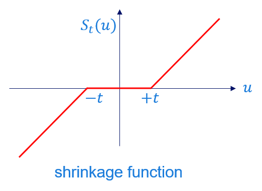
- if \(h(x) = t||x||_1\), then \(prox_t(x) = S_t(x)\), where \(S_t(x)\) is the shrinkage function defined as:
\[S_t(u) =
\begin{cases}
u-t & \quad \text{if } u>t\\
0 & \quad \text{if } |u|\leq t \\
u+t & \quad \text{if } u<-t\\
\end{cases}\]

- if \(h(X) = t||X||_\star\) where \( ||X||_\star \) is the nuclear norm of matrix \( X \) given by \( ||X||_\star = \sum_{i} \sigma_i(x)\) with \( \sigma_i(X) \) is the singular value of \( X \), the proximal operator for \( h(X) \) is:
\[prox_t(X) = U S_t(\Sigma) V^T\]
where, \( U, \Sigma, V \) are matrices obtained from SVD decomposition of matrix \( X \) i.e. \( X = U \Sigma V^T\) and \(S_t\) is the element-wise shringkage function defined as:
\[S_t(\Sigma) =
S_t\left( \begin{bmatrix}
\sigma_1 & 0 & \cdots & 0 \\
0 & \sigma_2 & \cdots & 0 \\
\vdots & \vdots & \ddots & \vdots \\
0 & 0 & \cdots & \sigma_N
\end{bmatrix} \right)
= \begin{bmatrix}
S_t(\sigma_1) & 0 & \cdots & 0 \\
0 & S_t(\sigma_2) & \cdots & 0 \\
\vdots & \vdots & \ddots & \vdots \\
0 & 0 & \cdots & S_t(\sigma_N)
\end{bmatrix}\]
We will give here few examples for application of the proximal operators:
LASSO
Consider a standard least square regresion problem with \(l_1\)-norm as:
\[\underset{\beta}{\text{minimize}}~\{f(\beta) = g(\beta) + h(\beta)\}\]
where, \( g(\beta) = \frac{1}{2}|| y-X\beta ||^2\) and \( h(\beta) = \lambda ||\beta||_1\) with \( y\in\mathbb{R}^n \), \( X \in\mathbb{R}^{n\times p} \) and \( \beta \in\mathbb{R}^p \).
The gradient of \( g(\beta) \) is: \( \nabla g(\beta) = X^T (X\beta - y)\)
The proximal operator of \( h(\beta) \) is: \( prox_\lambda(\beta) = S_\lambda (\beta)\)
This leads to the follwing “iterative shringkage thresholding algorithm” (ISTA):
- initialize at \( \beta_0 \)
- repeat until convergence: \( \beta_{k+1} = S_\lambda (\beta_k - t X^T (X\beta_k -y)) \)
Matrix completion
The matrix completion is usually stated as: Given a matrix \(A \in \mathbb{R}^{m\times n} \) with only \(P\) known elements. Under low-rank assumption of matrix \( A\), complete the missing elements.
Define \( \Phi: \mathbb{R}^{m\times n} \rightarrow \mathbb{R}^{m\times n} \) is a measurement operator with \( \left(\Phi A\right)_{(i,j)\in I} = A_{ij},~\left(\Phi A\right)_{(i,j)\notin I} = 0 \), \(I\) is the set of indices for known element of matrix \( A \) and \( | I | = P\).
The cost function for matrix completion problem is:
\[\begin{align*}
& \underset{X}{ \text{minimize}}~\{ f(X) = g(X) + h(X) \}\\
& g(X) = \frac{1}{2} \sum_{n=1}^{|I|} (X_{ij} - A_{ij})^2 = \frac{1}{2} || \Phi(X-A) ||^2 \\
& h(X) = \gamma ||X||_\star
\end{align*}\]
The gradient of \( g(X) \) is: \( \Phi(X-A) \)
The proximal operator of \( h(X) \) is: \( prox_\gamma(X) = S_\gamma (X)\)
This leads to the follwing matrix completion algorithm:
- initialize at \( X_0 \)
- repeat until convergence: \( X_{k+1} = S_\gamma (X_k - t_{k+1} \Phi (X_k - A)) \)