Introduction
The problem of our interest is the standard sparse linear regression:
\[y = H x +n\]
where \(y\in \mathbb{R}^M\) is the observation, \(x\in \mathbb{R}^N\) is the sparse signal, \(H\in \mathbb{R}^{M\times N} (M \ll N)\) is the known design matrix and \(n \in \mathbb{R}^N\) is the additive white Gaussian noise with zero mean and covariance \(\sigma^2\).
Iterative Soft Threshold Algorithm (ISTA)
This algorithm was discussed in detail in the previous post on the proximal gradient method.
The ISTA algorithm can be summarized as:
\[\begin{align*}
r^{(t)} &= \hat{x}^{(t)} + \alpha_t H^T (y-H \hat{x}^{(t)}) \\
\hat{x}^{(t+1)} &= \text{sign}(r^{(t)}) \text{max}\left( \left|r^{(t)}\right| -\alpha_t \lambda, 0\right)
\end{align*}\]
or, in an alternative form (here we set \(\alpha_t=1\) ):
\[\begin{align*}
z^{(t)} &= y - H \hat{x}^{(t)} \\
\hat{x}^{(t+1)} &= \eta\left( \hat{x}^{(t)} + H^T z^{(t)},\lambda \right)
\end{align*}\]
where,
\[\eta\left(x,\lambda\right) = \text{sign}(x) \text{max}\left(\left|x\right|, \lambda\right)\]
Approximate Message Passing
We provide here the Approximate Message Passing (AMP) algorithm:
\[\begin{align*}
z^{(t)} &= y - H \hat{x}^{(t)} + \frac{1}{\alpha} z^{(t-1)} \left\langle \eta^{\prime}_{t-1}\left( \hat{x}^{(t-1)} + H^T \hat{z}^{(t-1)} \right) \right\rangle\\
\hat{x}^{(t+1)} &= \eta_t\left( \hat{x}^{(t)} + H^T z^{(t)} \right)
\end{align*}\]
where, \( \langle x \rangle = \frac{1}{N} \sum_{i=1}^{N} x_i \) and \( \eta^\prime_{t-1} \) is the derivative of \( \eta_{t-1} \) is the Onsager correction term.
To derive the AMP algorithm, we start first with the reformulation of the above-mentioned sparse linear regression into a probabilistic inference problem with Laplace prior as below:
\[\begin{align*}
\hat{x} &= \underset{x}{\text{argmin}} \left( \frac{1}{2} \| y - H x\|_2^2 + \lambda \|x\|_1 \right) \\
&= \lim_{\beta\rightarrow \infty} \int x \frac{1}{Z_\beta} \exp\left( -\beta \left( \frac{1}{2} \| y - H x\|_2^2 + \lambda \|x\|_1 \right) \right)
\end{align*}\]
The probability term in the integration could be seen as the combination of two terms:
\[q(y|x) \propto \exp\left( -\frac{\beta}{2} \| y - H x\|_2^2 \right)\]
\[q(x) \propto \exp\left( -\beta \lambda \|x\|_1 \right)\]
The relation between variables \( \{x_i\}_{i=1}^{N} \) to constraints \( \{q(y_a|x)\}_{a=1}^{M} \) could be visualized via fractor graph below:
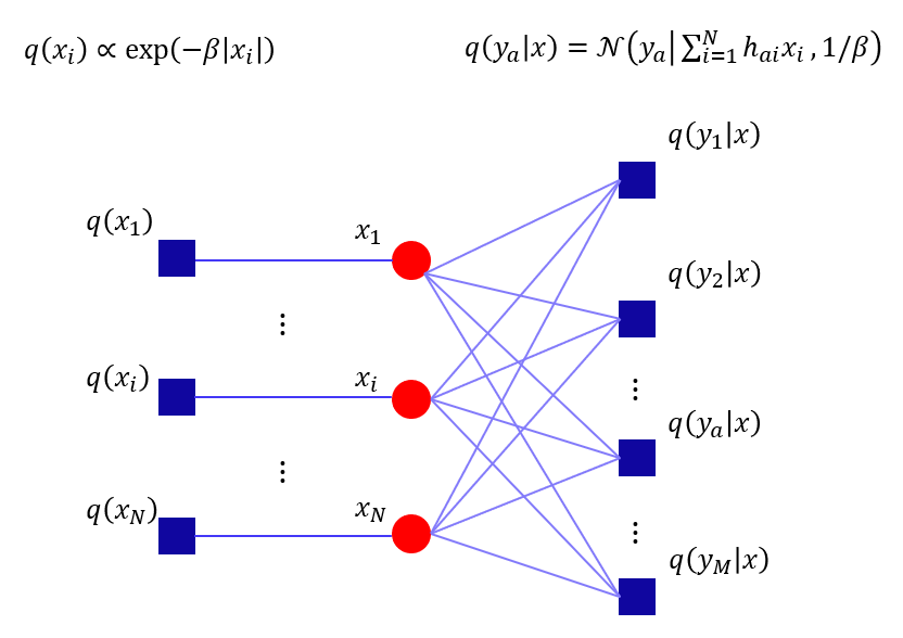
To calculate the posterior probability \( q(x_i|y) \), we use the message passing method for the factor graph:
\[\begin{align*}
\mu_{i\rightarrow a}^{(t+1)}(x_i) & \propto \exp\left(-\beta\lambda |x_i|\right) \prod_{b \neq a}^{M} \mu^{(t)}_{i \leftarrow b}(x_i) \\
\mu^{t}_{i \leftarrow a}(x_i) & \propto \int q(y_a|x) \prod_{j \neq i}^{N} \mu^{(t)}_{j \rightarrow a}(x_i) dx_{\backslash i}
\end{align*}\]
The posterior probability at time \( t+1 \) is given by:
\[\begin{align*}
q^{(t+1)}(x_i|y) & \propto \mu_{i}^{(t+1)}(x_i) \propto \mu_{i\rightarrow a}^{(t+1)}(x_i) \mu^{t}_{i \leftarrow a}(x_i) \\
q^{(t+1)}(x_i|y) & = \frac{ \exp\left(-\beta\lambda |x_i|\right) \prod_{a=1}^{M} \mu^{(t)}_{i \leftarrow a}(x_i) }{ \int \exp\left(-\beta\lambda |x_i|\right) \prod_{a=1}^{M} \mu^{(t)}_{i \leftarrow a}(x_i) dx_i }
\end{align*}\]
Consider the variable \( z_a = h_{ai} x_i + \sum_{j\neq i} h_{aj} x_j \), since \( \{x_i\}_{i=1}^{N} \) are i.i.d random variables, from (generalized) central limit theorem, when \(N\) is large, \(z_a\) is a Gaussian random variable with mean and variance at time \( t \) as:
\[\begin{align*}
\mathbb{E}[z_a] &= h_{ai} x_i + Z_{i\leftarrow a}^{(t)} \\
\text{var}[z_a] &= \frac{1}{\beta} V_{i\leftarrow a}^{(t)}
\end{align*}\]
where, \( Z^{(t)}_{i\leftarrow a} = \sum_{j\neq i} h_{aj} \hat{x}_{j\rightarrow a}^{t} \), \( V^{(t)}_{i\leftarrow a} = \sum_{j\neq i} |h_{aj}|^2 \hat{v}_{j\rightarrow a}^{t} \) and \( \hat{x}_{j\rightarrow a}^{t} \) and \( \hat{v}_{j\rightarrow a}^{t} \) are the mean vand variance of random variables \( x_j\) at time \(t\).
From this observation, we could simplify the expression for message \( \mu_{i\leftarrow a}^{(t)} \) as:
\[\begin{align*}
\mu^{t}_{i \leftarrow a}(x_i)
& \propto \int q(y_a|x) \prod_{j \neq i}^{N} \mu^{(t)}_{j \rightarrow a}(x_i) dx_{\backslash i} \\
& \propto \int_{x_{\backslash i}} \int_{z_a}\exp{\left(-\frac{\beta}{2} |y_a-z_a|^2 \right)} \delta\left( z_a - \sum_{k=1}^{N} h_{ak}x_k \right) \prod_{j \neq i}^{N} \mu^{(t)}_{j \rightarrow a}(x_i) dz_a dx_{\backslash i} \\
& \propto \int_{z_a}\exp{\left(-\frac{\beta}{2} |y_a-z_a|^2 \right)} \mathbb{E}\left[\delta\left( z_a - \sum_{j\neq i} h_{aj}x_j - h_{ai} x_i\right] \right) dz_a \\
&\overset{N\rightarrow \infty}{=} \int_{z_a}\exp{ \left( -\frac{\beta}{2} |y_a-z_a|^2 \right)} \mathcal{N}\left( z_a \middle| h_{ai} x_i + Z^{(t)}, \frac{1}{\beta} Z_{i\leftarrow a}^{(t)} \right) dz_a \\
& \propto \mathcal{N}\left( 0 \middle| y_a - h_{ai} x_i - Z^{(t)}_{i\leftarrow a}, \frac{1}{\beta}(1+V^{(t)}_{i\leftarrow a})\right) \\
& \propto \mathcal{N}\left( x_i \middle| \frac{y_a - Z^{(t)}_{i\leftarrow a}}{h_{ai}}, \frac{(1+V^{(t)}_{i\leftarrow a})}{\beta |h_{ai}|^2}\right)
\end{align*}\]
For later convenience, we denote \( \hat{x}_{i\leftarrow a}^{(t)} = \frac{y_a - Z^{(t)}_{i\leftarrow a}}{h_{ai}} \) and \( \hat{v}_{i\leftarrow a}^{(t)} = \frac{(1+V^{(t)}_{i\leftarrow a})}{\beta |h_{ai}|^2} \).
From the approximated result of \( \mu^{(t)}_{i\leftarrow a}\), we could calculate the message \( x^{(t+1)}_{i\leftarrow a}(x_i) \) as:
\[\begin{align*}
\mu_{i\rightarrow a}^{(t+1)}(x_i)
& \propto \exp\left(-\beta\lambda |x_i|\right) \prod_{b \neq a}^{M} \mu^{(t)}_{i \leftarrow b}(x_i) \\
& \propto \exp\left(-\beta\lambda |x_i|\right)~\mathcal{N}\left( x_i \middle| r^{(t)}_{i\rightarrow a}, \Sigma_{i\rightarrow a}^{(t)} \right)
\end{align*}\]
where,
\[\begin{align*}
\Sigma_{i\rightarrow a}^{(t)} &= \left( \sum_{b\neq a} \frac{|h_{bi}|^2}{1+V_{i\rightarrow b}^{(t)}} \right)^{-1}\\
r^{(t)}_{i\rightarrow a} &= \Sigma_{i\rightarrow a}^{(t)} \sum_{b\neq a} \frac{h_{bi}(y_b-Z^{(t)}_{i\leftarrow b})}{1+V^{(t)}_{i\leftarrow b}}
\end{align*}\]
For later convenience, we introduce some new functions:
\[\begin{align*}
f_{\beta}(x;r,\Sigma) &= \frac{1}{Z_{\beta}} \exp\left( -\beta\left( \lambda |x| + \frac{1}{2\Sigma}(x-r)^2 \right) \right) \\
F_\beta(x;r,\Sigma) &= \int x f_{\beta}(x;r,\Sigma) \\
G_\beta(x;r,\Sigma) &= \int x^2 f_{\beta}(x;r,\Sigma) - |F_\beta(x;r,\Sigma)|^2\\
\end{align*}\]
with this notations, we could rewrite the message as:
\[\mu_{i\rightarrow a}^{(t+1)}(x_i) =\mathcal{N}\left( x_i\middle| \hat{x}^{(t+1)}_{i\rightarrow a}, \hat{v}^{(t+1)}_{i\rightarrow a} \right)\]
where, \( \hat{x}^{(t+1)}_{i\rightarrow a} = F_\beta(x_i;r^{(t)}_{i\rightarrow a},\Sigma_{i\rightarrow a}^{(t)}) \) and \( \hat{v}^{(t+1)}_{i\rightarrow a} = \beta G_\beta(x_i;r^{(t)}_{i\rightarrow a},\Sigma_{i\rightarrow a}^{(t)})\)
We now have all necessary information to calculate the posterior probability:
\[\begin{align*}
q^{(t+1)}(x_i|y) &= \mathcal{N}\left( x_i\middle| \hat{x}^{(t+1)}_{i}, \hat{v}^{(t+1)}_{i} \right) \\
\hat{x}^{(t+1)}_{i} &= F_\beta(x_i;r^{(t)}_{i},\Sigma_{i}^{(t)}) \\
\hat{v}^{(t+1)}_{i} &= \beta G_\beta(x_i;r^{(t)}_{i},\Sigma_{i}^{(t)})\\
\Sigma_{i}^{(t)} &= \left( \sum_{a=1}^{M} \frac{|h_{ai}|^2}{1+V_{i\rightarrow a}^{(t)}} \right)^{-1}\\
r^{(t)}_{i} &= \Sigma_{i}^{(t)} \sum_{a=1}^{M} \frac{h_{ai} (y_a-Z^{(t)}_{i\leftarrow a})}{1+V^{(t)}_{i\leftarrow a}}
\end{align*}\]
Practical implementation with python
The tutorial solves the following LASSO problem:
\[\hat x=\arg\min_x\ \tfrac12\|y-Hx\|_2^2+\lambda\|x\|_1,\]
with \(y=Hx+n\), \(x\in\mathbb{R}^N\) sparse, \(H\in\mathbb{R}^{M\times N}\), \(M<N\). Three algorithms attack the same problem.
Soft-thresholding is the proximal operator of the \(\ell_1\) norm and the shared building block:
\[\eta(r,\theta)=\text{sign}(r)\,\max(|r|-\theta,0).\]
ISTA is plain proximal gradient descent. With step \(\alpha\) (stable iff \(\alpha<2/L\), where \(L=|H|_2^2\) is the Lipschitz constant of the smooth part):
\[x^{(t+1)}=\eta\!\big(x^{(t)}-\alpha H^\top(Hx^{(t)}-y),\ \alpha\lambda\big).\]
FISTA adds Nesterov momentum, extrapolating before the gradient step. This turns the \(O(1/t)\) rate of ISTA into \(O(1/t^2)\):
\[z^{(t)}=x^{(t)}+\tfrac{t-2}{t+1}\big(x^{(t)}-x^{(t-1)}\big),\qquad
x^{(t+1)}=\eta\!\big(z^{(t)}-\alpha H^\top(Hz^{(t)}-y),\ \alpha\lambda\big).\]
AMP is ISTA plus the Onsager correction. The residual carries a memory term built from the average denoiser derivative \(\langle\eta’\rangle\) (= the fraction of currently-active components):
\[\begin{aligned}
z^{(t)} &= y-Hx^{(t)} + \tfrac{1}{\delta}\,z^{(t-1)}\,\langle\eta'(x^{(t-1)}+H^\top z^{(t-1)})\rangle,\\
x^{(t+1)} &= \eta\!\big(x^{(t)}+H^\top z^{(t)},\ \theta_t\big),
\end{aligned}\]
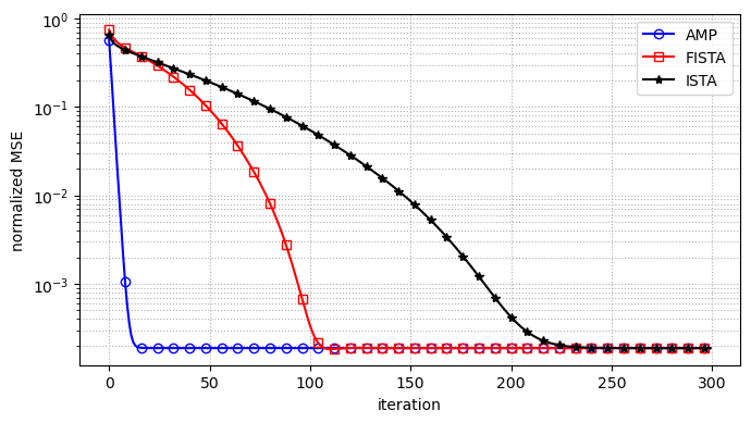
with \(\delta=M/N\). That one extra term decorrelates the residual so the denoiser always sees “signal + AWGN” (state evolution), which is why AMP needs an order of magnitude fewer iterations.
Signal model (Bernoulli–Gaussian): each entry of \(x\) is nonzero with probability \(\rho\) and, when nonzero, is \(\mathcal{N}(0,1/\rho)\); \(H\) has i.i.d. \(\mathcal{N}(0,1/M)\) entries; noise variance is set from the SNR via \(\nu_w=10^{-\text{SNR}_{\rm dB}/10}\).
Below is the self-contained python scripts that compares the convergence of AMP, FISTA and ISTA method:
"""
Approximate Message Passing (AMP) for the LASSO, compared with ISTA and FISTA.

this script compares AMP, FISTA, and ISTA on the LASSO-style problem

    minimize_x 0.5 ||y - A x||_2^2 + lambda ||x||_1,

where y = A x0 + noise and x0 is sparse.
"""

import numpy as np
import matplotlib.pyplot as plt

# problem generator: Bernoulli-Gaussian signal + Gaussian sensing matrix
def make_problem(N, M, rho, snr_dB, rng):
    """draw one instance of  y = H x + n."""
    # Bernoulli-Gaussian sparse signal: each entry nonzero with probability rho.
    x = np.sqrt(1.0 / rho) * rng.standard_normal(N)
    x *= (rng.random(N) < rho)

    # sensing matrix with entries ~ N(0, 1/M): columns are O(1)-normalized.
    H = rng.standard_normal((M, N)) / np.sqrt(M)

    nuw = 10.0 ** (-snr_dB / 10.0)          # noise variance from the SNR
    n = np.sqrt(nuw) * rng.standard_normal(M)
    y = H @ x + n
    return x, H, y

# soft-thresholding: the proximal operator of the l1 norm, eta(r, thr)
def soft(r, thr):
    return np.sign(r) * np.maximum(np.abs(r) - thr, 0.0)

def nmse(x_hat, x):
    return np.linalg.norm(x_hat - x) ** 2 / np.linalg.norm(x) ** 2

# ISTA: plain proximal gradient descent
def ista(H, y, x_true, lam, n_iter, step=None):
    N = H.shape[1]
    if step is None:
        step = 1.9 / np.linalg.norm(H, 2) ** 2 # just under the 2/L stability limit
    x_hat = np.zeros(N)
    mse = np.empty(n_iter)
    for t in range(n_iter):
        grad = H.T @ (H @ x_hat - y)
        x_hat = soft(x_hat - step * grad, lam * step)
        mse[t] = nmse(x_hat, x_true)
    return mse

# FISTA: ISTA + Nesterov momentum (with light damping for stability)
def fista(H, y, x_true, lam, n_iter, step=None, damp=0.85):
    N = H.shape[1]
    if step is None:
        step = 1.0 / np.linalg.norm(H, 2) ** 2 # 1/L: momentum needs the safe step
    x_prev = np.zeros(N)      # x^{(t-1)}
    x_prev2 = np.zeros(N)     # x^{(t-2)}
    x_damp = np.zeros(N)
    mse = np.empty(n_iter)
    for t in range(1, n_iter + 1):
        mom = (t - 2) / (t + 1) # Nesterov extrapolation weight
        z = x_prev + mom * (x_prev - x_prev2)
        grad = H.T @ (H @ z - y)
        x_hat = soft(z - step * grad, lam * step)
        mse[t - 1] = nmse(x_hat, x_true)
        x_hat = damp * x_hat + (1 - damp) * x_damp   # damping
        x_damp = x_hat
        x_prev2, x_prev = x_prev, x_hat
    return mse

# AMP: ISTA + Onsager correction term (the key ingredient)
def amp(H, y, x_true, lam, n_iter, damp=0.95):
    M, N = H.shape
    delta = M / N
    x_hat = np.zeros(N)
    z = np.zeros(M)
    z_old = np.zeros(M)
    onsager = np.zeros(M)
    gamma = 1.0 # effective extra threshold
    mse = np.empty(n_iter)
    for t in range(n_iter):
        # residual carrying the Onsager memory term.
        z = y - H @ x_hat + onsager
        z = damp * z + (1 - damp) * z_old  # damping for finite-size stability
        z_old = z

        thr = lam + gamma
        r = x_hat + H.T @ z
        x_hat = soft(r, thr)

        # <eta'> = fraction of components above threshold = average derivative.
        df = np.mean(np.abs(r) > thr)
        onsager = (1.0 / delta) * z * df   # Onsager reaction term
        gamma = thr / delta * df           # state-evolution threshold update

        mse[t] = nmse(x_hat, x_true)
    return mse

def main():
    N, M = 1024, 512
    rho = 0.05
    snr_dB = 50
    lam = 0.05
    n_iter = 300
    n_trials = 10

    rng = np.random.default_rng(0)
    acc = {"AMP": 0.0, "FISTA": 0.0, "ISTA": 0.0}
    for _ in range(n_trials):
        x, H, y = make_problem(N, M, rho, snr_dB, rng)
        acc["AMP"] += amp(H, y, x, lam, n_iter)
        acc["FISTA"] += fista(H, y, x, lam, n_iter)
        acc["ISTA"] += ista(H, y, x, lam, n_iter)
    for k in acc:
        acc[k] /= n_trials

    plt.figure(figsize=(7, 4))
    plt.semilogy(acc["AMP"], "-o", color="b", markevery=8, mfc="none", label="AMP")
    plt.semilogy(acc["FISTA"], "-s", color="r", markevery=8, mfc="none", label="FISTA")
    plt.semilogy(acc["ISTA"], "-*", color="k", markevery=8, label="ISTA")
    plt.xlabel("iteration")
    plt.ylabel("normalized MSE")
    plt.legend()
    plt.grid(True, which="both", ls=":")
    plt.tight_layout()
    plt.show()
    print("AMP   final NMSE:", acc["AMP"][-1])
    print("FISTA final NMSE:", acc["FISTA"][-1])
    print("ISTA  final NMSE:", acc["ISTA"][-1])


if __name__ == "__main__":
    main()
Results
All three methods reach the noise floor (\(\approx 1.9~10^{-4}\) at 50 dB SNR); AMP gets there around iteration 15, FISTA around 105, ISTA around 220.