For conventional kriging (also known as gaussian process regression), only one single output channel is considered in the modeling process.
In this note, we introduce the cokriging framework to be able to jointly model two different output channels. This technique is known as ‘multi-output gaussian process regression’ in machine learning community. Both ‘kriging’ and ‘cokriging’ terminology are from geostatistical community.
Consider a situation where we have two kinds of data:
- Primary data: \( \{ z_1(u_{\alpha_1}) \}_{\alpha_1 = 1 … n_1} \)
- Secondary data: \( \{ z_2(u_{\alpha_2}) \}_{\alpha_2 = 1 … n_2} \)
For practical reason, we only describe here the ordinary cokriging. Assuming \( z_1 \) and \( z_2 \) are realization of stationary random processes \( Z_1 \) with mean value \( m_1 \) and \( Z_2 \) with mean value \( m_2 \) respectively. The prediction of cokriging at the point \( u \) is given by:
\[Z^\ast_1(u) = \sum_{\alpha_1 = 1}^{n_1} \lambda_{\alpha_1}^{(1)}(u) Z_1(u_{\alpha_1}) + \sum_{\alpha_2 = 1}^{n_2} \lambda_{\alpha_2}^{(2)}(u) Z_2(u_{\alpha_2}) + \lambda_{m_1}(u) m_1 + \lambda_{m_2}(u) m_2\]
Since, \( \mathbb{E}[Z_1(u_{\alpha_1})] = \mathbb{E}[Z^\ast_1(u)] = m_1 \) and \( \mathbb{E}[Z_2(u_{\alpha_2})] = m_2 \), then we have:
\[\begin{align*}
\lambda_{m_1} &= 1 - \sum_{\alpha_1=1}^{n_1} \lambda_{\alpha_1}^{(1)}(u) \\
\lambda_{m_2} &= - \sum_{\alpha_2=1}^{n_2} \lambda_{\alpha_2}^{(2)}(u)
\end{align*}\]
To remove the need for mean estimation, we set \( \lambda_{m_1} = 0 \) and \( \lambda_{m_2} = 0 \), this leads to:
\[\begin{cases}
Z^\ast_1(u) & = \sum_{\alpha_1 = 1}^{n_1} \lambda_{\alpha_1}^{(1)}(u) Z_1(u_{\alpha_1}) + \sum_{\alpha_2 = 1}^{n_2} \lambda_{\alpha_2}^{(2)}(u) Z_2(u_{\alpha_2})\\
\sum_{\alpha_1=1}^{n_1} \lambda_{\alpha_1}^{(1)}(u) & = 1 \\
\sum_{\alpha_2=1}^{n_2} \lambda_{\alpha_2}^{(2)}(u) & = 0
\end{cases}\]
The criteria to find the best estimator is to minimize the following variance:
\[\begin{align*}
\sigma_E^2(u) & = \text{var}\left[ Z^\ast_1(u) - Z_1(u)\right] \\
& = \text{var}\left[ \sum_{\alpha_1 = 1}^{n_1} \lambda_{\alpha_1}^{(1)}(u) Z_1(u_{\alpha_1}) + \sum_{\alpha_2 = 1}^{n_2} \lambda_{\alpha_2}^{(2)}(u) Z_2(u_{\alpha_2}) - Z_1(u)\right] \\
& = \sum_{\alpha_1,\alpha_1'} \lambda_{\alpha_1}^{(1)} \lambda_{\alpha_1'}^{(1)} \text{cov}\left[ Z_1(u_{\alpha_1}), Z_1(u_{\alpha_1'})\right] + \sum_{\alpha_2,\alpha_2'} \lambda_{\alpha_2}^{(2)} \lambda_{\alpha_2'}^{(2)} \text{cov}\left[ Z_2(u_{\alpha_2}), Z_2(u_{\alpha_2'})\right] + 2\sum_{\alpha_1,\alpha_2} \lambda_{\alpha_1}^{(1)} \lambda_{\alpha_2}^{(2)} \text{cov}\left[ Z_1(u_{\alpha_1}), Z_2(u_{\alpha_2})\right] \\
& ~ + \text{var}\left[ Z_1(u) \right] - 2\sum_{\alpha_1 = 1}^{n_1} \lambda_{\alpha_1}^{(1)}(u) \text{var}\left[ Z_1(u_{\alpha_1}), Z_1(u) \right] - 2\sum_{\alpha_2 = 1}^{n_2} \lambda_{\alpha_2}^{(2)}(u) \text{var}\left[ Z_2(u_{\alpha_2}), Z_1(u) \right]
\end{align*}\]
The Lagrangian for this problem is:
\[\mathcal{L}(u) = \sigma_E^2(u) + 2\mu_1 \left( \sum_{\alpha_1=1}^{n_1} \lambda_{\alpha_1}^{(1)}(u) - 1 \right) + 2\mu_2 \left( \sum_{\alpha_2=1}^{n_2} \lambda_{\alpha_2}^{(2)}(u) \right)\]
The best estimator should correspond to following system of equations:
\[\begin{cases}
\frac{1}{2} \frac{\partial \mathcal{L}}{\partial \lambda^{(i)}_{\alpha_i}} & = 0 ~~~ \text{for}~ i = 1, 2 \\
\frac{1}{2} \frac{\partial \mathcal{L}}{\partial \mu_i} & = 0 ~~~ \text{for}~ i = 1, 2
\end{cases}\]
Since \( Z_1 \) and \( Z_2 \) are stationary processes, we could define the covariance and cross-covariance as follows:
\[\begin{cases}
\text{cov}\left[ Z_1(u_{\alpha_1}), Z_1(u_{\beta_1}) \right] & = C_{11} (u_{\alpha_1} - u_{\beta_1}) \\
\text{cov}\left[ Z_2(u_{\alpha_2}), Z_2(u_{\beta_2}) \right] & = C_{22} (u_{\alpha_2} - u_{\beta_2}) \\
\text{cov}\left[ Z_1(u_{\alpha_1}), Z_2(u_{\beta_2}) \right] & = C_{12}(u_{\alpha_1} - u_{\beta_2}) \\
\text{cov}\left[ Z_2(u_{\alpha_2}), Z_1(u_{\beta_1}) \right] & = C_{21}(u_{\alpha_2} - u_{\beta_1})
\end{cases}\]
The system of equations is rewrote in term of covariances and cross-covariances as follows:
\[\begin{cases}
\sum_{\beta_1 = 1}^{n_1} \lambda_{\beta_1}^{(1)}(u) C_{11}(u_{\alpha_1} - u_{\beta_1}) + \sum_{\beta_2 = 1}^{n_2} \lambda_{\beta_2}^{(2)}(u) C_{12}(u_{\alpha_1} - u_{\beta_2}) + \mu_1(u) & = C_{11}(u_{\alpha_1}) - u ~~~ \text{for}~ \alpha_1 = 1 ... n_1 \\
\sum_{\beta_1 = 1}^{n_1} \lambda_{\beta_1}^{(1)}(u) C_{21}(u_{\alpha_2} - u_{\beta_1}) + \sum_{\beta_2 = 1}^{n_2} \lambda_{\beta_2}^{(2)}(u) C_{22}(u_{\alpha_2} - u_{\beta_2}) + \mu_2(u) & = C_{21}(u_{\alpha_2}) - u ~~~ \text{for}~ \alpha_2 = 1 ... n_2 \\
\sum_{\alpha_1=1}^{n_1} \lambda_{\alpha_1}^{(1)}(u) & = 1 \\
\sum_{\alpha_2=1}^{n_2} \lambda_{\alpha_2}^{(2)}(u) & = 0
\end{cases}\]
The variance of estimator at the optimal solution is:
\[\begin{align*}
\sigma^2(u) & = C_{11}(0) - \mu_1(u) - \sum_{\alpha_1=1}^{n_1} \lambda_{\alpha_1}^{(1)}(u) C_{11}(u_{\alpha_1} - u) - \sum_{\alpha_2=1}^{n_2} \lambda_{\alpha_2}^{(2)}(u) C_{21}(u_{\alpha_2} - u) \\
& = - \mu_1(u) + \sum_{\alpha_1=1}^{n_1} \lambda_{\alpha_1}^{(1)}(u) (C_{11}(0)-C_{11}(u_{\alpha_1} - u)) + \sum_{\alpha_2=1}^{n_2} \lambda_{\alpha_2}^{(2)}(u) (C_{21}(0)-C_{21}(u_{\alpha_2} - u)) \\
& = - \mu_1(u) + \sum_{\alpha_1=1}^{n_1} \lambda_{\alpha_1}^{(1)}(u) \gamma_{11}(u_{\alpha_1} - u) + \sum_{\alpha_2=1}^{n_2} \lambda_{\alpha_1}^{(2)}(u) \gamma_{21}(u_{\alpha_2} - u)
\end{align*}\]
here, we introduce the notion of (cross-) variogram \( \gamma_{ij}(h) = C_{ij}(0) - C_{ij}(h)\).
In matrix notation, the optimal estimator can be found via solving the following equation:
\[\begin{pmatrix}
\mathbf{K}_{1,1} & \mathbf{K}_{1,2} & \mathbf{1}_1 & \mathbf{0}_1 \\
\mathbf{K}_{2,1} & \mathbf{K}_{2,2} & \mathbf{0}_2 & \mathbf{1}_2 \\
\mathbf{1}_1^T & \mathbf{0}_2^T & 0 & 0 \\
\mathbf{0}_1^T & \mathbf{1}_2^T & 0 & 0
\end{pmatrix}
\begin{pmatrix}
\boldsymbol{\lambda}_1(u) \\
\boldsymbol{\lambda}_2(u) \\
\mu_1(u) \\
\mu_2(u)
\end{pmatrix}
=\begin{pmatrix}
\mathbf{k}_{11} \\
\mathbf{k}_{21} \\
1 \\
0
\end{pmatrix}\]
where,
\[\begin{align*}
\mathbf{K}_{11} & = \left[ C_{11}(u_{\alpha_1}-u_{\beta_1}) \right]_{\alpha_1 = 1 ... n_1, \beta_1 = 1 ... n_1} \\
\mathbf{K}_{22} & = \left[ C_{22}(u_{\alpha_2}-u_{\beta_2}) \right]_{\alpha_2 = 1 ... n_2, \beta_1 = 1 ... n_2} \\
\mathbf{K}_{21} & = \left[ C_{21}(u_{\alpha_2}-u_{\beta_1}) \right]_{\alpha_2 = 1 ... n_2, \beta_1 = 1 ... n_1} \\
\mathbf{K}_{12} & = \left[ C_{12}(u_{\alpha_1}-u_{\beta_2}) \right]_{\alpha_1 = 1 ... n_1, \beta_2 = 1 ... n_2} \\
\boldsymbol{\lambda}_1(u) & =
\begin{pmatrix}
\lambda_1^{(1)}(u) \\
\lambda_2^{(1)}(u) \\
\vdots \\
\lambda_{n_1}^{(1)}(u)
\end{pmatrix} \\
\boldsymbol{\lambda}_2(u) & =
\begin{pmatrix}
\lambda_1^{(2)}(u) \\
\lambda_2^{(2)}(u) \\
\vdots \\
\lambda_{n_2}^{(2)}(u)
\end{pmatrix}\\
\mathbf{k}_{11} & =
\begin{pmatrix}
C_{11}(u_1-u) \\
C_{11}(u_2-u) \\
\vdots \\
C_{11}(u_{n_1}-u)
\end{pmatrix}\\
\mathbf{k}_{21} & =
\begin{pmatrix}
C_{21}(u_1-u) \\
C_{21}(u_2-u) \\
\vdots \\
C_{21}(u_{n_2}-u)
\end{pmatrix}
\end{align*}\]
The prediction of cokriging at new location \( u \) is given by:
\[\begin{align*}
Z_1^\ast(u) & = \sum_{\alpha_1 = 1}^{n_1} \lambda_{\alpha_1}^{(1)}(u) Z_1(u_{\alpha_1}) + \sum_{\alpha_2 = 1}^{n_2} \lambda_{\alpha_2}^{(2)}(u) Z_2(u_{\alpha_2})\\
& =
\begin{pmatrix}
\mathbf{Z}_{1}^T(u) & \mathbf{Z}^T_{2}(u) & 0 & 0
\end{pmatrix}
\begin{pmatrix}
\boldsymbol{\lambda_1}^{(1)}(u) \\
\boldsymbol{\lambda_2}^{(1)}(u) \\
\mu_1(u) \\
\mu_2(u)
\end{pmatrix}\\
& =
\begin{pmatrix}
\mathbf{Z}_{1}(u) & \mathbf{Z}_{2}(u) & 0 & 0
\end{pmatrix}
\begin{pmatrix}
\mathbf{K}_{1,1} & \mathbf{K}_{1,2} & \mathbf{1}_1 & \mathbf{0}_1 \\
\mathbf{K}_{2,1} & \mathbf{K}_{2,2} & \mathbf{0}_2 & \mathbf{1}_1 \\
\mathbf{1}_1^T & \mathbf{0}_2^T & 0 & 0 \\
\mathbf{0}_1^T & \mathbf{1}_2^T & 0 & 0
\end{pmatrix}^{-1}
\begin{pmatrix}
\mathbf{k}_{11} \\
\mathbf{k}_{21} \\
1 \\
0
\end{pmatrix}
\end{align*}\]
Theoretical variogram models
The theoretical variogram \( 2\gamma (h) \) of an ‘intrinsic’ stationary process \( Z(u) \) is defined as:
\[2\gamma (h) = \text{var}[Z(u+h)-Z(u)]\]
Since the covarinace is given by \( C(h) = \mathbb{E}[Z(u)Z(u+h)] - \mu^2\) with \(\mu = \mathbb{E}[Z(u)]\), then we have:
\[\gamma (h) = C(0) - C(h)\]
The standard definition of cross-variogram is:
\[2\gamma_{ij} = \mathbb{E}[(Z_i(u+h)-Z_i(u))(Z_j(u+h)-Z_j(u))]\]
Linear Model of Coregionalization
Within the linear model of coregionalization framework, each stationary function \( Z_i(u) \) is a linear combination of independent stationary function \( Y_k^l(u) \) with zero mean and covariance \(c_l(h)\) as below:
\[Z_i(u) = \sum_{l=1}^{L} \sum_{k=1}^{N_l} a_{ik}^l Y_k^l(u) + m_i ~~~ \forall i\]
From this definition, we can deduce the relation between the (cross-) covariance of \(Z_i(u)\) and the covariances of independent stationary functions \(c_l(h)\) as:
\[C_{ij}(h) = \sum_{l=1}^{L} \left( \sum_{k=1}^{N_l} a_{ik}^l a_{jk}^l\right) c_l(h) = \sum_{l=1}^L b_{ij}^l c_i(h)\]
With \(c_l(h)\) are permissible covariance models, the sufficient condition for \(C_{ij}(h)\) to be a permisssible model of coregionalization is that all the coregionalization matrices \( B_l = [b_{ij}^l] \) are positive simi-definite.
Cokriging in practice: a python/pytorch tutorial
In this section, we build ordinary cokriging from scratch on a 1D toy problem: numpy for the data and the kriging systems, pytorch for fitting the variogram model by gradient descent. The full python script is provided in this github repository cokriging_1d. The MATLAB version can be found via this link.
The setting: a primary variable measured sparsely (only on part of the domain) and a secondary variable that is cheap to measure and densely sampled everywhere. Because the two are correlated, the secondary data should improve the prediction of the primary one - that is the whole point of cokriging.
Background needed for the implementation
The theory post derives the cokriging system in terms of covariances \(C_{ij}\). Three practical ingredients are still missing before we can write code.
1. From covariances to variograms
Implementations usually work with variograms \(\gamma_{ij}(h) = C_{ij}(0) - C_{ij}(h)\) rather than covariances, because the empirical variogram is easier to estimate (it does not require knowing the means). The two formulations give the same weights: substitute \(C_{ij} = C_{ij}(0) - \gamma_{ij}\) into the cokriging system and use the constraints:
\[\begin{aligned}
\sum_{\alpha_1} \lambda^{(1)}_{\alpha_1} &= 1,\\
\sum_{\alpha_2} \lambda^{(2)}_{\alpha_2} &= 0;
\end{aligned}\]
all the \(C_{ij}(0)\) terms either cancel or are absorbed into the Lagrange multipliers (which flip sign). The system we solve in the code is therefore
\[\begin{pmatrix}
\boldsymbol{\Gamma}_{11} & \boldsymbol{\Gamma}_{12} & \mathbf{1} & \mathbf{0} \\
\boldsymbol{\Gamma}_{21} & \boldsymbol{\Gamma}_{22} & \mathbf{0} & \mathbf{1} \\
\mathbf{1}^T & \mathbf{0}^T & 0 & 0 \\
\mathbf{0}^T & \mathbf{1}^T & 0 & 0
\end{pmatrix}
\begin{pmatrix}
\boldsymbol{\lambda}_1 \\ \boldsymbol{\lambda}_2 \\ \mu_1 \\ \mu_2
\end{pmatrix}
=\begin{pmatrix}
\boldsymbol{\gamma}_{11}(u) \\ \boldsymbol{\gamma}_{21}(u) \\ 1 \\ 0
\end{pmatrix}\]
with \([\boldsymbol{\Gamma}_{ij}]_{\alpha\beta} = \gamma_{ij}(u_\alpha - u_\beta)\),
and the prediction and variance are
\[Z_1^\ast(u) = \boldsymbol{\lambda}_1^T \mathbf{Z}_1 + \boldsymbol{\lambda}_2^T \mathbf{Z}_2,
\qquad
\sigma^2(u) = \boldsymbol{\lambda}_1^T \boldsymbol{\gamma}_{11}(u) + \boldsymbol{\lambda}_2^T \boldsymbol{\gamma}_{21}(u) + \mu_1 .\]
2. Empirical (cross-)variograms
The classical (Matheron) estimator bins all data pairs by their separation \(h\):
\[\hat\gamma_{ii}(h) = \frac{1}{2 |N(h)|} \sum_{(\alpha,\beta) \in N(h)} \left( z_i(u_\alpha) - z_i(u_\beta) \right)^2,\]
where \(N(h)\) is the set of pairs whose distance falls in the bin around \(h\). The cross-variogram estimator replaces the squared difference by the product of the increments of the two variables,
\[\hat\gamma_{12}(h) = \frac{1}{2 |N(h)|} \sum_{(\alpha,\beta) \in N(h)} \left( z_1(u_\alpha) - z_1(u_\beta) \right) \left( z_2(u_\alpha) - z_2(u_\beta) \right),\]
and therefore needs both variables at the same locations - in the code we keep only the collocated points. Practical rules: ignore lags beyond half the maximum distance (too few pairs), skip empty bins, and - when the data sit on a regular grid - make sure all pairs with the same nominal lag land in the same bin. The last point is easy to get wrong: floating-point jitter in \(|x_i - x_j|\) splits equal-lag pairs across two adjacent bins whenever a lag coincides with a bin edge, and since the two subsets are position-correlated their means can differ a lot (the empirical variogram then shows a spurious “two-branch” pattern). Rounding the distances before binning fixes it.
3. Nugget effect and a valid coregionalization model
Measurement noise shows up as a nugget: a jump of the variogram at the origin, \(\gamma_{ii}(h) = c_{0,i} + \text{(continuous part)}\) for \(h > 0\), with \(\gamma_{ii}(0) = 0\). If the noises on the two variables are independent, the cross-variogram has no nugget. In the kriging matrix the nugget appears on all off-diagonal entries of the diagonal blocks (and on the right-hand side, since a prediction point is not a data point) - this is exactly a Gaussian noise term in GP language.
For the continuous part we use a one-structure linear model of coregionalization (LMC):
\[\gamma_{ij}(h) = B_{ij}\, \gamma_m(h; \ell) + \delta_{ij}\, c_{0,i},
\qquad
\gamma_m(h) = 1 - \left( 1 + \frac{\sqrt 5 h}{\ell} + \frac{5 h^2}{3 \ell^2} \right) e^{-\sqrt 5 h / \ell},\]
i.e. a Matérn-5/2 variogram with unit sill shared by all three (cross-)variograms, scaled by a coregionalization matrix \(B\). The model is valid iff \(B \succeq 0\). In the MATLAB version this is enforced with a nonlinear constraint \(B_{12}^2 \le B_{11} B_{22}\) inside fmincon; in pytorch there is a neater trick - parametrize \(B = L L^T\) with \(L\) lower-triangular (positive diagonal via softplus). Then \(B\) is positive semi-definite by construction and the fit becomes an unconstrained problem that plain Adam can handle. We use the Matérn-5/2 closed form rather than the general-\(\nu\) Matérn because the latter needs the modified Bessel function \(K_\nu\), which is not available (differentiably) in pytorch.
Implementation
Step 1 - toy data
Two noisy, phase-shifted cosines. The primary variable is only observed on \([0, 0.6]\); the secondary one covers \([0, 1]\).
import numpy as np
import torch
import matplotlib.pyplot as plt

rng = np.random.default_rng(12345)

X1 = np.arange(0.0, 0.6 + 1e-9, 0.02)   # primary: sparse, partial coverage
X2 = np.arange(0.0, 1.0 + 1e-9, 0.01)   # secondary: dense, full coverage

Y1 = np.cos(2 * np.pi * X1 + 1.5) + 0.03 * rng.standard_normal(X1.shape)
Y2 = np.cos(2 * np.pi * X2 + 1.0) + 0.03 * rng.standard_normal(X2.shape)
Step 2 - empirical variograms
def empirical_variogram(X, Y, n_bins=20):
    """binned semivariogram: gamma(h) = 0.5 * E[(Z(u+h) - Z(u))^2]."""
    dist = np.abs(X[:, None] - X[None, :]).ravel()
    sqdiff = ((Y[:, None] - Y[None, :]) ** 2).ravel()
    return _bin_variogram(dist, 0.5 * sqdiff, n_bins)

def empirical_cross_variogram(X1, Y1, X2, Y2, n_bins=20):
    """gamma_12(h) = 0.5 * E[(Z1(u+h) - Z1(u)) (Z2(u+h) - Z2(u))],
    computed on collocated points only."""
    i1, i2 = np.nonzero(np.isclose(X1[:, None], X2[None, :]))
    Xc, Y1c, Y2c = X1[i1], Y1[i1], Y2[i2]
    dist = np.abs(Xc[:, None] - Xc[None, :]).ravel()
    cross = ((Y1c[:, None] - Y1c[None, :]) * (Y2c[:, None] - Y2c[None, :])).ravel()
    return _bin_variogram(dist, 0.5 * cross, n_bins)

def _bin_variogram(dist, gam, n_bins):
    # round distances so that pairs with the same nominal lag always fall in
    # the same bin (see background section 2).
    dist = np.round(dist, 9)
    # only use lags up to half the maximum distance (few pairs beyond that)
    edges = np.linspace(0, dist.max() / 2, n_bins + 1)
    h, g = [], []
    for lo, hi in zip(edges[:-1], edges[1:]):
        sel = (dist >= lo) & (dist < hi) & (dist > 0)
        if sel.sum() > 0:
            h.append(0.5 * (lo + hi))
            g.append(gam[sel].mean())
    return np.array(h), np.array(g)

h11, g11 = empirical_variogram(X1, Y1)                  # primary
h22, g22 = empirical_variogram(X2, Y2)                  # secondary
h12, g12 = empirical_cross_variogram(X1, Y1, X2, Y2)    # cross
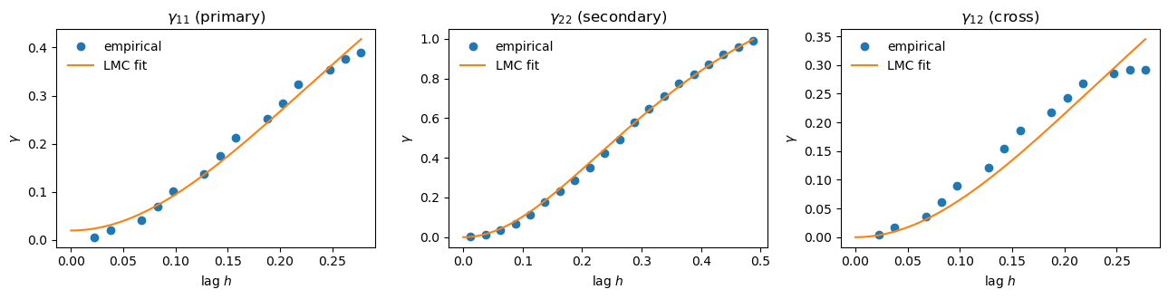
A remark on data quality: the primary window \([0, 0.6]\) covers barely more than half a period of the cosine, so its empirical variogram is necessarily noisy - averaging over positions is a poor substitute for averaging over realizations when the signal is periodic and the window short (the process is far from ergodic at these lags). The dense secondary variogram is much cleaner, which is precisely why borrowing its structure through the cross-variogram pays off.
Step 3 - fit the LMC with pytorch
The only trainable objects are the raw Cholesky factor of \(B\), the log-scale length \(\ell\), and the two nuggets. The loss is the sum of mean-squared errors between the three model variograms and their empirical counterparts - the same least-squares criterion as the MATLAB version, but with no constraint, thanks to the Cholesky parametrization. A few random restarts guard against bad local minima.
def matern52_vario(h, ell):
    """Matern nu=5/2 variogram with unit sill."""
    s = np.sqrt(5.0) * h / ell
    return 1.0 - (1.0 + s + s ** 2 / 3.0) * torch.exp(-s)

def lmc_variograms(params, h11, h22, h12):
    raw_L, raw_ell, raw_c0 = params
    ell = torch.nn.functional.softplus(raw_ell)
    c0 = torch.nn.functional.softplus(raw_c0) # nuggets (noise)
    L = torch.tril(raw_L)
    L = L - torch.diag(torch.diag(L)) \
          + torch.diag(torch.nn.functional.softplus(torch.diag(raw_L)))
    B = L @ L.T # PSD by construction
    return (B[0, 0] * matern52_vario(h11, ell) + c0[0],
            B[1, 1] * matern52_vario(h22, ell) + c0[1],
            B[0, 1] * matern52_vario(h12, ell)), B, ell, c0

t = lambda a: torch.as_tensor(a, dtype=torch.float64)
th11, tg11, th22, tg22, th12, tg12 = map(t, (h11, g11, h22, g22, h12, g12))

best = {"loss": np.inf}
for restart in range(5):
    torch.manual_seed(restart)
    params = [torch.randn(2, 2, dtype=torch.float64, requires_grad=True),        # raw_L
              (0.5 * torch.rand(1, dtype=torch.float64) - 1.5).requires_grad_(), # raw_ell
              torch.full((2,), -6.0, dtype=torch.float64, requires_grad=True)]   # raw nuggets
    opt = torch.optim.Adam(params, lr=0.05)
    for step in range(1500):
        opt.zero_grad()
        (m11, m22, m12), *_ = lmc_variograms(params, th11, th22, th12)
        loss = ((m11 - tg11) ** 2).mean() + ((m22 - tg22) ** 2).mean() \
             + ((m12 - tg12) ** 2).mean()
        loss.backward()
        opt.step()
    if loss.item() < best["loss"]:
        best = {"loss": loss.item(), "params": [p.detach().clone() for p in params]}

with torch.no_grad():
    _, B, ell, c0 = lmc_variograms(best["params"], th11, th22, th12)
B, ell, c0 = B.numpy(), ell.item(), c0.numpy()

def gamma_model(h, i, j):
    """fitted variogram model gamma_ij at lag(s) h (NumPy in, NumPy out)."""
    with torch.no_grad():
        g = float(B[i, j]) * matern52_vario(t(h), t(ell)).numpy()
    return g + (c0[i] if i == j else 0.0) * (np.asarray(h) > 0)
Note how the nugget multiplies (h > 0): the model variogram is exactly zero at zero lag, and jumps to \(c_{0,i}\) for any positive lag - this single line takes care of all the noise bookkeeping in the kriging matrices below.
Step 4 - ordinary kriging (baseline) and ordinary cokriging
Both are “build matrix, solve, dot with data”. Kriging on the primary data alone:
Xt = np.linspace(0.0, 1.0, 200)
n1, n2, nt = len(X1), len(X2), len(Xt)

def solve(A, b):
    try:
        return np.linalg.solve(A, b)
    except np.linalg.LinAlgError:
        return np.linalg.lstsq(A, b, rcond=None)[0]

D11 = np.abs(X1[:, None] - X1[None, :])
A = gamma_model(D11, 0, 0)
A = np.block([[A, np.ones((n1, 1))], [np.ones((1, n1)), np.zeros((1, 1))]])
b = np.vstack([gamma_model(np.abs(X1[:, None] - Xt[None, :]), 0, 0),
               np.ones((1, nt))])
lam = solve(A, b)
Y_krig = lam[:n1].T @ Y1
S_krig = np.sqrt(np.maximum((lam * b).sum(axis=0), 0))
Cokriging stacks the two data sets and adds one unbiasedness constraint per output (\(\sum \boldsymbol{\lambda}_1 = 1\), \(\sum \boldsymbol{\lambda}_2 = 0\)):
D22 = np.abs(X2[:, None] - X2[None, :])
D12 = np.abs(X1[:, None] - X2[None, :])

G = np.block([[gamma_model(D11, 0, 0), gamma_model(D12, 0, 1)],
              [gamma_model(D12.T, 0, 1), gamma_model(D22, 1, 1)]])
e1 = np.concatenate([np.ones(n1), np.zeros(n2)])
e2 = np.concatenate([np.zeros(n1), np.ones(n2)])
A = np.block([[G, e1[:, None], e2[:, None]],
              [e1[None, :], np.zeros((1, 2))],
              [e2[None, :], np.zeros((1, 2))]])
b = np.vstack([gamma_model(np.abs(X1[:, None] - Xt[None, :]), 0, 0),
               gamma_model(np.abs(X2[:, None] - Xt[None, :]), 0, 1),
               np.ones((1, nt)),
               np.zeros((1, nt))])
lam = solve(A, b)
Y_cokrig = lam[:n1 + n2].T @ np.concatenate([Y1, Y2])
S_cokrig = np.sqrt(np.maximum((lam * b).sum(axis=0), 0))
The prediction variance \(\boldsymbol{\lambda}^T \boldsymbol{\gamma}(u) + \mu_1\) is conveniently just (lam * b).sum(axis=0), because the Lagrange rows of b are \((1, 0)\).
Step 5 - results
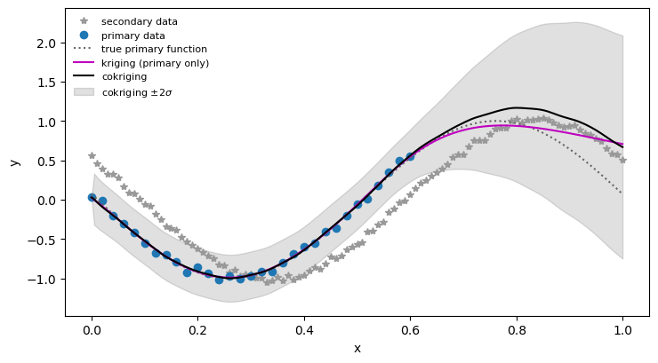
On \([0, 0.6]\), where primary data exist, kriging and cokriging agree. Beyond \(x = 0.6\) ordinary kriging has no information and relaxes to the data mean, while cokriging keeps tracking the shape of the densely-sampled secondary variable - with a variance that stays finite because the cross-correlation is imperfect.
Below is the plot from variogram/cross-variogram fitting (to determine model parameters):
And the final result for cokriging vs kriging is shown in the following plot:
- Connection to multi-output GPs. What we built is exactly a two-task GP with an ICM/LMC kernel \(K((x,i),(x’,j)) = B_{ij} k_m(x,x’) + \delta_{ij} \sigma_i^2\), plus an improper uniform prior on per-task constant means (that is what the ordinary-kriging constraints amount to). The variogram-fitting step replaces maximum-likelihood training; libraries such as GPyTorch (
MultitaskKernel) do the same thing with MLE and would be the natural next step for higher dimensions or more outputs.
- Method-of-moments vs MLE. Variogram fitting is robust and visualizable (you can see whether the model fits), but uses only binned second moments. MLE uses all the data jointly and handles irregular/heterotopic designs without a collocation step - at the price of \(O((n_1+n_2)^3)\) per gradient step and less interpretability.
- More structures. The LMC with \(L > 1\) structures (e.g. Matérn + nugget + long-range component) is the direct generalization: \(\gamma_{ij}(h) = \sum_l B^{(l)}_{ij} \gamma_l(h)\), one Cholesky-parametrized \(B^{(l)}\) per structure. The code above is the \(L = 1\) special case.