Sparse Gaussian Processes
Assuming a dataset \( (X,y) \) of \(N\) training samples, building a Gaussian process requires an inversion of \(N\times N\) matrix which takes \( \mathcal{O}(N^3) \) time.
The idea of sparse GP with inducing points (SPGP) is to replace the original data with a smaller dataset \( (Z, u = f(Z)) \) where \( f \) is the true latent function.
The likelihood with the inducing points are:
\[\begin{aligned}
\mathbb{P}(y|X,Z,u,\theta) & = \prod_{n=1}^N \mathbb{P}(y_n|x_n,Z,\theta)\\
& = \prod_{n=1}^N \mathcal{N}(y_n|K_{f_n u}K_{uu}^{-1}u, K_{f_n f_n}, K_{f_n f_n} - K_{f_n u} K_{uu}^{-1}K_{u f_n} + \sigma^2)\\
& = \mathcal{N}(y|K_{fu}K_{uu}^{-1}u, K_{ff}, \text{diag}(K_{ff} - Q_{ff}) + \sigma^2\mathbb{I})
\end{aligned}\]
where, \( Q_{ff} = K_{fu} K_{uu}^{-1}K_{uf}\)
By placing the prior for \(u\) as \( \mathbb{P}(u|Z,\theta) = \mathcal{N}(u|0,K_{u u})\) as it is the output of the true latent function \(f\), we can simplify the likelihood as:
\[\begin{aligned}
\mathbb{P}(y|X,Z) & = \int \mathbb{P}(y|X,Z,u,\theta) \mathbb{P}(u|Z,\theta) du\\
& = \mathcal{N}(y|0,Q_{ff} + \text{diag}(K_{ff}-Q_{ff}) + \sigma^2\mathbb{I})
\end{aligned}\]
The inducing inputs \(Z\) is obtained via maximing the likelihood function \( \mathbb{P}(y|X,Z) \).
To obtain the prediction at new data points \(X_\star,y_\star\), we start first with the joint distribution \(\mathbb{P}(y,y_\star|X,X_\star,Z)\) and then calculate the conditioned probablity \( \mathbb{P}(y_\star|y,X,X_\star,Z)\). This leads to:
\[\begin{aligned}
\mathbb{P}(y_\star|y,X,X_\star,Z) & = \mathcal{N}(y_\star|\mu_\star,\Sigma_\star)~~\text{where}\\
\mu_\star & = Q_{\star f}\left(Q_{ff} + \text{diag}(K_{ff}-Q_{ff}) + \sigma^2\mathbb{I}\right)^{-1}y\\
\Sigma_\star & = K_{\star\star} - Q_{\star f}\left(K_{ff}-Q_{ff}) + \sigma^2\mathbb{I}\right)^{-1} Q_{f\star}
\end{aligned}\]
A C++ implementation of SPGP can be found in the github repo SPGP tutorial.
Deep Gaussian Processes
Deep Gaussian Processes assume that data is generated via a composition of multiple Gaussian Processes as:
\[y = f_L( f_{L-1}( \cdots ( f_1(X) )\cdots ) ) + \epsilon\]
where, \(f_l\) is drawn from a Gaussian Process.
We define new notations for later calculations: \( h_l = f_l( f_{l-1}( \cdots ( f_1(X) )\cdots ) ) + \epsilon_l\), \( h_L = y\) and \( h_0 = X \)
The joint probability between intermediate value \(\{h_l\}_{l}\) and the outputs \(y\) is:
\[\begin{aligned}
\mathbb{P}(y,h_1, ..., h_{L-1}|X) & = \mathbb{P}(y|h_L) \prod_{l=1}^{L-1} \mathbb{P}(h_l | h_{l-1})\\
\mathbb{P}(y|f_L) & = \mathcal{N}(f_L,\sigma_n^2 \mathbb{I})\\
\mathbb{P}(h_l|h_{l-1}) & = \mathcal{N}(0,K_{h_l h_l} + \sigma_l^2 \mathbb{I})
\end{aligned}\]
The joint probability is difficult to estimate. To circumvent this problem, we will use the Gaussian approximation techniques. We will focus on the ‘nested variational approach’ (see Hensman and Lawrence, 2014).
In the nested variational approach, to avoid the computational cost of large dataset, following the sparse Gaussian Process approach, a set of inducing points \( \{Z_l, u_l = f_l(Z_l)\}_{l} \) is introduced for layer \(l\).
For convenience, we drop the \(X, Z\) in the conditioned probablity expression e.g. \( \mathbb{P}(y|u, X, Z)\) is reduced to \( \mathbb{P}(y|u)\).
For the first layer, the variational lower bound is given by:
\[\begin{aligned}
\log \mathbb{P}(h_1|u_1) & = \log \int \mathbb{P}(h_1|f_1) \mathbb{P}(f_1|u_1) df_1\\
& \overset{(a)}{\geq} \int \mathbb{P}(f_1|u_1) \log \mathbb{P}(h_1|f_1) df_1\\
& \overset{(b)}{=} \int \mathbb{P}(f_1|u_1) \left( -\frac{N}{2} \log 2\pi \sigma^2_1 - \frac{1}{2\sigma_1^2} (h_1-f_1)^T(h_1-f_1) \right) df_1\\
& \geq \log \mathcal{N}(h1|K_{h_1 u_1}K_{u_1 u_1}^{-1} m_1, \sigma_1^2 \mathbb{I}) - \text{tr}\left(K_{h_1 u_1} K_{u_1 u_1}^{-1} S_1 K_{u_1 u_1}^{-1} K_{u_1 h_1} \right)\\
& \overset{\Delta}{=} \log \tilde{\mathbb{P}}(h_1|u_1)
\end{aligned}\]
Notes:
\( (a) \): here, we use Jensen’s inequality \( \log \mathbb{E}(f(X)) \geq \mathbb{E}(\log f(X)) \)
\( (b) \): from definition, we have \( \mathbb{P}(h_1|f_1) = \mathcal{N}(h_1|f_1, \sigma_1^2 \mathbb{I}) \) and sparse Gaussian Process formulation, we have \( \mathbb{P}(f_1|u_1) = \mathcal{N}(f_1|K_{h_1 u_1}K_{u_1 u_1}^{-1} u_1, K_{h_1 h_1} - K_{h_1 u_1}K_{u_1 u_1}^{-1}K_{u_1 h_1} ) \overset{\Delta}{=} \mathcal{N}(h_1|\mu_1, \Sigma_1)\)
The inequality for \( \mathbb{P}(h_1|u_1) \) can be generalized for other layers and this leads to:
\[\mathbb{P}(y, h_1, ..., h_{L-1}|X, u_1, ..., u_L) \geq \prod_{l=1}^{L} \tilde{\mathbb{P}}(h_l | u_l, h_{l-1}) \exp\left(-\sum_{l=1}^{L} \frac{1}{\sigma_l^2} \text{tr}(\Sigma_l)\right)\]
where, \( \log \tilde{\mathbb{P}}(h_l|u_l, h_{l-1}) = \mathcal{N}(h_l|\mu_l, \sigma_l^2 \mathbb{I}) \), \( \mu_l = K_{h_l u_l}K_{u_l u_l}^{-1} u_l\) and \(\Sigma_l = K_{h_l h_l} - K_{h_l u_l}K_{u_l u_l}^{-1}K_{u_l h_l}\).
For the second layer, we give below the detailed derivation of the variational lower bound. First, we choose the variational distributions \( Q(u_l) = \mathcal{N}(u_l|m_l, S_l) \) and \( Q(h_l) = \int Q(u_l) \tilde{\mathbb{P}}(h_l|u_l, h_{l-1}) du_l\).
\[\begin{aligned}
\log \mathbb{P}(h_2|u_2,u_1) & = \log \int \mathbb{P}(h_2,h_1|u_2,u_1) dh_1\\
& \geq \log \int \tilde{\mathbb{P}}(h_2|u_2,h_1) \tilde{\mathbb{P}}(h_1|u_1) \exp\left(-\frac{1}{2\sigma_1^2} \text{tr}(\Sigma_1)\right) \exp\left(-\frac{1}{2\sigma_2^2} \text{tr}(\Sigma_2)\right) dh_1\\
& \overset{(a)}{\geq} \mathbb{E}_{\tilde{\mathbb{P}}(h_1|u_1)}\left[\log \tilde{\mathbb{P}}(h_2|u_2,h_1) \right] - \mathbb{E}_{\tilde{\mathbb{P}}(h_1|u_1)}\left[ \frac{1}{2\sigma_2^2} \text{tr}(\Sigma_2) \right] - \frac{1}{2\sigma_1^2} \text{tr}(\Sigma_1)
\end{aligned}\]
Notes:
\( (a) \): here, we use Jensen’s inequality \( \log \mathbb{E}(f(X)) \geq \mathbb{E}(\log f(X)) \)
By marginalizing the variable \( u_1 \) using the variational distribution \( Q(u_1) \), we have:
\[\begin{aligned}
\log \mathbb{P}(h_2|u_2) & = \log \int \mathbb{P}(h_2,u_1|u_2) du_1\\
& = \log \int \mathbb{P}(h_2|u_1,u_2) \mathbb{P}(u_1) du_1\\
& \geq \int Q(u_1) \log \frac{\mathbb{P}(h_2|u_1,u_2) \mathbb{P}(u_1)}{Q(u_1)} du_1\\
& = \mathbb{E}_{Q(u_1)}\left[\mathbb{P}(h_2|u_1,u_2)\right] - \text{KL}\left[Q(u_1)\|\mathbb{P}(u_1)\right]\\
& \geq \mathbb{E}_{Q(u_1)}\left[ \mathbb{E}_{\tilde{\mathbb{P}}(h_1|u_1)}\left[\log \tilde{\mathbb{P}}(h_2|u_2,h_1) \right] \right] - \text{KL}\left[Q(u_1)\|\mathbb{P}(u_1)\right]\\
& ~~~~~ - \mathbb{E}_{Q(u_1)}\left[\mathbb{E}_{\tilde{\mathbb{P}}(h_1|u_1)}\left[ \frac{1}{2\sigma_2^2} \text{tr}(\Sigma_2) \right]\right]- \frac{1}{2\sigma_1^2} \text{tr}(\Sigma_1) \\
& = \mathbb{E}_{Q(h_1)}\left[\log \tilde{\mathbb{P}}(h_2|u_2,h_1) \right] - \text{KL}\left[Q(u_1)\|\mathbb{P}(u_1)\right] - \mathbb{E}_{Q(h_1)}\left[ \frac{1}{2\sigma_2^2} \text{tr}(\Sigma_2) \right] - \frac{1}{2\sigma_1^2} \text{tr}(\Sigma_1)
\end{aligned}\]
Using the analytical form of \( Q(h_1) = \mathcal{N}(h_1|m_1, S_1)\) and direct calculation, we obtain the variational lower bound for \( \log \mathbb{P}(h_2|u_2)\) as:
\[\begin{aligned}
\log \mathbb{P}(h_2|u_2) \geq & \log \mathcal{N}(h_2|\Psi_2 K_{u_2 u_2}^{-1} m_2, \sigma_2^2\mathbb{I}) - \text{KL}(Q(u_1)||\mathbb{P(u_1)})\\
& -\frac{1}{2\sigma_1^2} \text{tr}\left(K_{11}-Q_{11}\right) - \frac{1}{2\sigma_2^2}\left(\psi_2 - \text{tr}(\Psi_2 K_{u_2 u_2}^{-1})\right)\\
& -\frac{1}{2\sigma_2^2} \text{tr}\left((\Phi_2-\Psi_2^T \Psi_2) K_{u_2 u_2}^{-1} u_2 u_2^T K_{u_2 u_2}^{-1}\right)
\end{aligned}\]
where,
\[\begin{aligned}
\psi_2 & = \mathbb{E}_{Q(h_1)} \left[ \text{tr}(K_{h_2 h_2}) \right]\\
\Psi_2 & = \mathbb{E}_{Q(h_1)} \left[ K_{h_2 u_2} \right]\\
\Phi_2 & = \mathbb{E}_{Q(h_1)} \left[ K_{u_2 h_2} K_{h_2 u_2} \right]
\end{aligned}\]
By applying the similar steps for other layers, we obtain the nested variational compression lower bound as:
\[\begin{aligned}
\log \mathbb{P}(y|X) & = \log \int \mathbb{P}(y|u_L,X) \mathbb{P}(u_L) du_L\\
& \geq \int \mathbb{P}(u_L) \log \mathbb{P}(y|u_L, X) du_L\\
& \geq \log \mathcal{N}(y|\Psi_L K_{u_L u_L}^{-1} m_L, \sigma_n^2\mathbb{I}) - \sum_{l=1}^L \text{KL}(Q(u_l)||\mathbb{P(u_l)})\\
& -\frac{1}{2\sigma_1^2} \text{tr}\left(K_{11}-Q_{11}\right) - \sum_{l=2}^L \frac{1}{2\sigma_l^2}\left(\psi_l - \text{tr}(\Psi_l K_{u_l u_l}^{-1})\right)\\
& -\sum_{l=2}^L \frac{1}{2\sigma_l^2} \text{tr}\left((\Phi_l-\Psi_l^T \Psi_l) K_{u_l u_l}^{-1} (m_l m_l^T+S_l) K_{u_l u_l}^{-1}\right)
\end{aligned}\]
here, similarly to the calculation of \( \log \mathbb{P}(h_2|u_2) \), we introduce new parameters as
\[\begin{aligned}
\psi_l & = \mathbb{E}_{Q(h_{l-1})} \left[ \text{tr}(K_{h_l h_l}) \right]\\
\Psi_l & = \mathbb{E}_{Q(h_{l-1})} \left[ K_{h_l u_l} \right]\\
\Phi_l & = \mathbb{E}_{Q(h_{l-1})} \left[ K_{u_l h_l} K_{h_l u_l} \right]
\end{aligned}\]
Note also that \( m_l m_l^T + S_l \) is the explicit result of \( \mathbb{E}_{Q(h_l)}[u_l u_l^T] \) with \( Q(h_l) = \mathcal{N}(h_l|m_l, S_l) \).
Doubly Stochastic Deep Gaussian Processes
This note has two parts: first, what “doubly stochastic” DGP inference (Salimbeni & Deisenroth, NeurIPS 2017, arXiv:1705.08933) is and how it differs from the nested variational compression; second, a self-contained ~150-line PyTorch implementation (no GPflow/GPyTorch) is provided.
Part 1 - The doubly stochastic DGP
Setup
\[y = f_L(f_{L-1}(\cdots f_1(X)\cdots)) + \epsilon,\qquad f_l \sim \mathcal{GP}\]
Each layer gets inducing points \({Z_l, u_l = f_l(Z_l)}\) and a variational distribution \(q(u_l) = \mathcal{N}(m_l, S_l)\). So far identical to nested variational compression.
The key simplification
The variational posterior over everything is chosen as
\[q(\{f_l, u_l\}_{l=1}^L) = \prod_{l=1}^{L} \underbrace{p(f_l \mid u_l; h_{l-1}, Z_l)}_{\text{exact GP conditional}}\; q(u_l)\]
Two things to notice. First, the only free variational parameters are \({m_l, S_l, Z_l}\) - the conditionals \(p(f_l|u_l)\) are kept exact, not approximated. Second, and crucially, \(q\) does not assume independence between layers: \(f_l\) depends on the actual output \(h_{l-1}\) of the layer below. Marginalizing \(u_l\) analytically gives, for each layer,
\[q(f_l \mid h_{l-1}) = \mathcal{N}\!\left(\mu_l(h_{l-1}),\, \Sigma_l(h_{l-1})\right)\]
with the standard sparse-GP equations (\(\mu_l = K_{h u}K_{uu}^{-1}m_l\) and \(\Sigma_l = K_{hh} - K_{hu}K_{uu}^{-1}(K_{uu}-S_l)K_{uu}^{-1}K_{uh}\)).
The ELBO and the two sources of stochasticity
The bound has exactly the same shape as single-layer SVGP (Hensman et al., 2013):
\[\mathcal{L} = \sum_{n=1}^{N} \mathbb{E}_{q(f_L^{(n)})}\!\left[\log p(y_n \mid f_L^{(n)})\right] \;-\; \sum_{l=1}^{L} \mathrm{KL}\!\left[q(u_l)\,\|\,p(u_l)\right]\]
The expectation \(q(f_L^{(n)})\) - the marginal of the final layer at input \(x_n\) - is intractable (it’s a continuous mixture of Gaussians through the layers). But it depends only on the \(n\)-th input: within each layer the marginals factorize over data points. So you can sample it cheaply with the reparameterization trick:
\[\hat{h}_l^{(n)} = \mu_l(\hat{h}_{l-1}^{(n)}) + \sqrt{\Sigma_l(\hat{h}_{l-1}^{(n)})}\;\varepsilon_l^{(n)},\qquad \varepsilon \sim \mathcal{N}(0, I)\]
i.e. propagate each data point through the stack, sampling layer by layer, and evaluate the likelihood term at the end. Gradients flow through the samples.
The two “doubly” stochastic parts:
- Monte-Carlo sampling of the intractable expectation through the layers (reparameterized, so it’s differentiable).
- Minibatching: the likelihood term is a sum over \(n\), so subsample and rescale by \(N/|\mathcal{B}|\).
Contrast with nested variational compression:
| |
Nested variational compression (Hensman & Lawrence ‘14) |
Doubly stochastic (Salimbeni & Deisenroth ‘17) |
| Inter-layer coupling |
Cut: \(q(h_l)\) approximated as Gaussian between layers |
Kept: samples carry the full dependence |
| Expectations over layers |
Analytic \(\psi_l, \Psi_l, \Phi_l\) statistics |
Monte Carlo |
| Kernel restrictions |
Needs closed-form \(\Psi\)-statistics (essentially RBF/linear) |
Any kernel |
| Likelihood restrictions |
Gaussian (for the closed forms) |
Any (just needs \(\log p(y|f)\) evaluable) |
| Extra bound-loosening terms |
Trace correction terms at every layer |
None beyond standard SVGP-style bound |
| Implementation |
Heavy algebra |
~150 lines, autodiff does the work |
The practical lesson from the paper: the sampling approach is simpler and tighter - every Jensen application you did per layer loosens the bound, while the MC estimate is unbiased for the single-Jensen bound above. That’s why the doubly stochastic formulation became the standard DGP baseline.
Two implementation details from the paper that matter in practice:
- Whitened parameterization. Parameterize \(q(v)\) with \(u = \mathrm{chol}(K_{zz})\,v\), so the prior on \(v\) is \(\mathcal{N}(0,I)\). The KL becomes the trivial \(\mathrm{KL}[\mathcal{N}(m,S)|\mathcal{N}(0,I)]\) and optimization is much better conditioned.
- Identity/linear mean functions for inner layers. With zero mean functions, a deep GP prior collapses towards flat functions (Duvenaud et al., 2014). Salimbeni & Deisenroth give inner layers the identity (or a PCA-style linear map when dimensions differ) as mean function, so at initialization the whole stack is close to the identity and behaves like a single GP. Initialize \(S_l \approx 10^{-5} I\) for inner layers so early training is nearly deterministic.
Prediction
Propagate test points through the layers by sampling \(S\) times; the predictive density is the Gaussian mixture \(\frac{1}{S}\sum_s \mathcal{N}!\left(y_\star \mid \mu_L^{(s)}, \Sigma_L^{(s)} + \sigma^2\right)\).
Part 2 - From-scratch PyTorch tutorial
Below is the whole algorithm with no GP library. Everything fits in four small classes. The full script can be found in the github repository.
2.1 Kernel
class RBFKernel(torch.nn.Module):
    """k(x,x') = s2 * exp(-|x-x'|^2 / (2 l^2)), ARD lengthscales."""

    def __init__(self, input_dim, lengthscale=1.0, variance=1.0):
        super().__init__()
        self.log_lengthscale = torch.nn.Parameter(
            math.log(lengthscale) * torch.ones(input_dim))
        self.log_variance = torch.nn.Parameter(torch.tensor(math.log(variance)))

    def K(self, X, X2=None):
        X2 = X if X2 is None else X2
        Xs = X / self.log_lengthscale.exp()
        X2s = X2 / self.log_lengthscale.exp()
        d2 = (Xs**2).sum(-1, keepdim=True) - 2 * Xs @ X2s.mT \
            + (X2s**2).sum(-1).unsqueeze(-2)
        return self.log_variance.exp() * torch.exp(-0.5 * d2.clamp_min(0.0))

    def K_diag(self, X):
        return self.log_variance.exp().expand(X.shape[:-1])
Note the batch-friendly shapes: X can be (S, N, D) - sample dimension in front - and everything broadcasts.
2.2 The sparse variational GP layer
The heart of the method. Whitened: \(q(v) = \mathcal{N}(m, LL^\top)\), \(u = \mathrm{chol}(K_{zz})v\). With \(A = \mathrm{chol}(K_{zz})^{-1}K_{zx}\):
\[\mu = A^\top m, \qquad \mathrm{diag}\,\Sigma = k_{\mathrm{diag}} - \mathrm{diag}(A^\top A) + \mathrm{diag}(A^\top L L^\top A)\]
class SVGPLayer(torch.nn.Module):
    def __init__(self, kernel, Z, out_dim, mean_function=None):
        super().__init__()
        self.kernel = kernel
        M = Z.shape[0]
        self.Z = torch.nn.Parameter(Z.clone())
        self.q_mu = torch.nn.Parameter(torch.zeros(M, out_dim))
        self.q_sqrt = torch.nn.Parameter(
            1e-5 * torch.eye(M).expand(out_dim, M, M).clone())
        self.mean_function = mean_function  # None => zero mean

    def conditional(self, X):
        """q(f(X)) marginals. X: (..., N, D_in) -> mean, var: (..., N, D_out)."""
        Kzz = self.kernel.K(self.Z) + JITTER * torch.eye(len(self.Z))
        Lz = torch.linalg.cholesky(Kzz)
        Kzx = self.kernel.K(self.Z, X)                           # (..., M, N)
        A = torch.linalg.solve_triangular(Lz, Kzx, upper=False)  # whitened
        mean = A.mT @ self.q_mu                                  # (..., N, D_out)
        SA = self.q_sqrt.mT @ A.unsqueeze(-3)                    # (..., D_out, M, N)
        var = (self.kernel.K_diag(X).unsqueeze(-1)
               - (A**2).sum(-2, keepdim=True).mT
               + (SA**2).sum(-2).movedim(-2, -1))                # (..., N, D_out)
        if self.mean_function is not None:
            mean = mean + self.mean_function(X)
        return mean, var.clamp_min(1e-10)

    def sample(self, X):
        """reparameterized sample from q(f(X))."""
        mean, var = self.conditional(X)
        return mean + var.sqrt() * torch.randn_like(mean)

    def KL(self):
        """KL[q(v)||N(0,I)], summed over output dims."""
        L = torch.tril(self.q_sqrt)
        trace = (L**2).sum((-1, -2))
        logdet = torch.log(L.diagonal(dim1=-2, dim2=-1)**2).sum(-1)
        quad = (self.q_mu**2).sum(0)
        M = self.q_mu.shape[0]
        return 0.5 * (trace + quad - M - logdet).sum()
2.3 The deep GP: propagate by sampling
class DeepGP(torch.nn.Module):
    def __init__(self, layers, noise_var=0.1):
        super().__init__()
        self.layers = torch.nn.ModuleList(layers)
        self.log_noise = torch.nn.Parameter(torch.tensor(math.log(noise_var)))

    def propagate(self, X, num_samples=5):
        """draw S samples of the final-layer marginals q(f_L)."""
        F = X.expand(num_samples, *X.shape)
        for layer in self.layers[:-1]:
            F = layer.sample(F)
        return self.layers[-1].conditional(F)  # mean, var: (S, N, D_out)

    def elbo(self, X, y, num_samples=5, num_data=None):
        num_data = num_data if num_data is not None else len(X)
        mean, var = self.propagate(X, num_samples)
        s2 = self.log_noise.exp()
        # E_{q(f)}[log N(y|f, s2)] in closed form per sample:
        lik = (-0.5 * math.log(2 * math.pi) - 0.5 * s2.log()
               - 0.5 * ((y - mean)**2 + var) / s2)
        lik = lik.mean(0).sum()               # average samples, sum data
        kl = sum(layer.KL() for layer in self.layers)
        return (num_data / len(X)) * lik - kl
This is the entire algorithm:
propagate is the doubly stochastic trick - F has shape (S, N, D) and each layer call resamples.- In
elbo, note we don’t sample the last layer: for a Gaussian likelihood, \(\mathbb{E}_{\mathcal{N}(f|\mu,v)}[\log\mathcal{N}(y|f,\sigma^2)] = \log\mathcal{N}(y|\mu,\sigma^2) - \frac{v}{2\sigma^2}\) is closed-form (that’s the variational_expectations call in GPflow). One less variance source.
(num_data / len(X)) is the minibatch rescaling - the second “stochastic”.
2.4 Prediction
@torch.no_grad()
def predict(self, X, num_samples=100):
    """moments of the predictive mixture (1/S) sum_s N(m_s, v_s + s2)."""
    mean, var = self.propagate(X, num_samples)
    var = var + self.log_noise.exp()
    m = mean.mean(0)
    v = (var + mean**2).mean(0) - m**2   # law of total variance
    return m, v
The predictive is a mixture of Gaussians, so it can be multi-modal and have non-Gaussian marginals - one of the genuine payoffs of depth. The moment-matched m, v is convenient for plotting, but for log-likelihood evaluation use logsumexp over the mixture components.
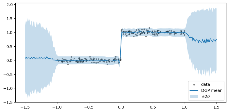
2.5 Demo: step function
N = 200
X = torch.rand(N, 1) * 2 - 1
y = (X > 0).double() + 0.05 * torch.randn(N, 1)

Z = torch.linspace(-1, 1, 25).unsqueeze(-1)
model = make_dgp([1, 1, 1], Z)   # 2-layer DGP, identity mean inside

opt = torch.optim.Adam(model.parameters(), lr=0.01)
for step in range(2000):
    opt.zero_grad()
    loss = -model.elbo(X, y, num_samples=5)
    loss.backward()
    opt.step()
A step function is the canonical DGP demo: a stationary single-layer GP must trade off “sharp at 0” against “smooth elsewhere” with a single lengthscale; the 2-layer model learns a first layer that compresses the input space around the discontinuity, so the second layer sees an easy problem. The result of deep gaussian process is shown below:
References
- Ed Snelson & Zoubin Ghahramani (2005), Sparse Gaussian processes using pseudo-inputs, NeurIPS 2005
- Salimbeni & Deisenroth (2017), Doubly Stochastic Variational Inference for Deep Gaussian Processes, arXiv:1705.08933
- Hensman & Lawrence (2014), Nested Variational Compression in Deep Gaussian Processes, arXiv:1412.1370
- Hensman, Fusi & Lawrence (2013), Gaussian Processes for Big Data (SVGP)
- Damianou & Lawrence (2013), Deep Gaussian Processes
- Duvenaud, Rippel, Adams & Ghahramani (2014), Avoiding pathologies in very deep networks