Topology optimization asks a deceptively simple question: given a design domain, boundary conditions, and a material budget, what is the stiffest structure you can build? The density-based SIMP method is the best-known answer (see for example, the classic “99-line” tutorial or the updated “88-line” tutorial), but there is an older and mathematically richer one: treat the shape itself as the optimization variable and differentiate with respect to it. That is Hadamard’s boundary variation method, dating back to 1907, turned into a practical algorithm by the level-set framework of Allaire, Jouve and Toader (2004) and Wang, Wang and Guo (2003).
This post, which originated from my work on (photonics) inverse design, explains the technical content of the tutorial code piece by piece: the shape derivative, why it lives only on the boundary, how a Hamilton-Jacobi equation turns it into an algorithm, and the numerical details that make the loop stable.
1. The model problem
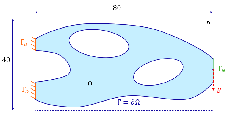
We work in a rectangular box \(D = [0,80] \times [0,40]\) holding a cantilever (see figure below): the left edge is clamped, and a unit point load \(g\) pulls down at the middle of the right edge. The structure is an open set \(\Omega \subset D\), and the displacement \(u\) solves linear elasticity on \(\Omega\):
\[-\,\mathrm{div}\big(A\,e(u)\big) = 0 \ \text{in } \Omega, \qquad
u = 0 \ \text{on } \Gamma_D, \qquad
A\,e(u)\,n = g \ \text{on } \Gamma_N, \qquad
A\,e(u)\,n = 0 \ \text{on } \Gamma,\]
where \(e(u) = \tfrac12(\nabla u + \nabla u^T)\) is the strain, \(A\) the Hooke tensor (plane stress, \(E=1\), \(\nu = 0.3\)), \(\Gamma_D\) the clamped edge, \(\Gamma_N\) the loaded part, and \(\Gamma\) the free boundary - the only part the optimizer may move.
The objective is compliance, the work done by the load:
\[J(\Omega) = \int_{\Gamma_N} g \cdot u \, ds = \int_\Omega A\,e(u) : e(u)\, dx,\]
minimized subject to a volume constraint \(|\Omega| = V_{\text{target}}\). Minimizing compliance means maximizing stiffness for a fixed amount of material. (Here, \(A:B\) is the Frobenius inner product between tensors/matrices/vectors \(A\) and \(B\)).
2. Hadamard’s boundary variation
To differentiate \(J\) with respect to \(\Omega\) we need a notion of “perturbing a shape.” Hadamard’s idea is to deform the domain by a smooth vector field \(\theta : \mathbb{R}^2 \to \mathbb{R}^2\):
\[\Omega_\theta = (\mathrm{Id} + \theta)(\Omega).\]
For small \(\theta\), \(\mathrm{Id} + \theta\) is a diffeomorphism, so \(\Omega_\theta\) is a genuine deformed copy of \(\Omega\) - points of the domain are transported by \(\theta\). A functional \(J\) is shape differentiable at \(\Omega\) if
\[J(\Omega_\theta) = J(\Omega) + J'(\Omega)(\theta) + o(\|\theta\|),\]
with \(J’(\Omega)\) linear and continuous in \(\theta\). This is just a Fréchet derivative, but in the unusual Banach space \(W^{1,\infty}(\mathbb{R}^2;\mathbb{R}^2)\) of deformation fields.
The key result is the Hadamard structure theorem: for smooth enough \(\Omega\), the derivative depends only on the normal trace of \(\theta\) on the boundary,
\[J'(\Omega)(\theta) = \int_{\partial\Omega} v\, (\theta \cdot n)\, ds,\]
for some scalar function \(v\) on \(\partial\Omega\) called the shape gradient. The intuition: a tangential \(\theta\) merely reparametrizes the boundary without changing the set, so it cannot change \(J\) to first order. All the information needed for a gradient descent is one scalar field on the boundary - this single fact is what the entire algorithm exploits.
3. The shape derivative of compliance
Computing \(v\) for compliance is a classical exercise in adjoint analysis (Céa’s method is the quickest route). Compliance is self-adjoint: the adjoint state turns out to be \(p = -u\), so no extra PDE solve is needed. The result, for variations supported on the traction-free boundary \(\Gamma\), is
\[J'(\Omega)(\theta) = -\int_{\Gamma} A\,e(u) : e(u)\, (\theta \cdot n)\, ds.\]
The integrand \(A\,e(u):e(u)\) is twice the elastic energy density - a nonnegative quantity. The sign tells the whole story: pushing the boundary outward (\(\theta \cdot n > 0\)) always decreases compliance, and it decreases it most where the material is working hardest. Of course, growing everywhere violates the volume budget, so we introduce a Lagrange multiplier \(\ell\) and minimize \(L(\Omega) = J(\Omega) + \ell\,|\Omega|\). Since the shape derivative of volume is \(\int_\Gamma \theta\cdot n \, ds\),
\[L'(\Omega)(\theta) = \int_{\Gamma} \big(\ell - A\,e(u):e(u)\big)\, (\theta \cdot n)\, ds.\]
A steepest-descent choice is now obvious: take the normal velocity
\[v_n = \theta \cdot n = A\,e(u):e(u) - \ell,\]
which gives \(L’(\Omega)(\theta) = -\int_\Gamma v_n^2\, ds \le 0\). The physical reading is an economic one: \(\ell\) is the price of material. Where the energy density exceeds the price, the boundary grows; where material earns less than it costs, the boundary recedes.
4. From boundary motion to a Hamilton-Jacobi equation
A descent step means moving every boundary point along its normal with speed \(v_n\). Tracking a moving curve explicitly (with markers or a boundary mesh) is fragile - curves merge, holes vanish, corners form. The level-set method of Osher and Sethian sidesteps all of it. Represent the shape implicitly:
\[\Omega = \{x \in D : \phi(x) < 0\}, \qquad \partial\Omega = \{\phi = 0\},\]
with \(\phi > 0\) in the void. The outward normal is \(n = \nabla\phi / |\nabla\phi|\). If the front moves with normal speed \(v_n\), the level-set function satisfies the Hamilton-Jacobi transport equation
\[\frac{\partial \phi}{\partial t} + v_n\, |\nabla \phi| = 0.\]
A short derivation: a point \(x(t)\) on the front satisfies \(\phi(x(t),t)=0\) and \(\dot x = v_n n\); differentiating in \(t\) gives \(\partial_t\phi + v_n\, n\cdot\nabla\phi = \partial_t\phi + v_n|\nabla\phi| = 0\).
Two things make this representation powerful here. First, \(v_n = A\,e(u):e(u) - \ell\) extends naturally off the boundary - the energy density is defined everywhere in \(D\) - so the equation can be solved on the whole grid with no interface extraction. Second, topological changes are free: when two holes merge or a thin bar pinches off, \(\phi\) stays perfectly smooth even though \(\partial\Omega\) changes topology. Each instant of the evolution is a pure Hadamard boundary variation; the level-set transport simply composes infinitely many of them, and topology transitions happen in passing. (One genuine limitation remains: in 2D the evolution cannot nucleate new holes in the interior, which is why the initial design is seeded with holes. The topological derivative is the standard remedy; we do not need it for a tutorial.)
5. The ersatz material trick
The shape derivative formula assumes a PDE posed on \(\Omega\) with a traction-free boundary \(\Gamma\). Re-meshing \(\Omega\) at every iteration would be costly and brittle. Instead the elasticity problem is solved on the fixed grid covering all of \(D\), with the void filled by a very soft “ersatz” material:
\[\rho_e = \varepsilon_{\text{void}} + (1 - \varepsilon_{\text{void}})\,\mathrm{frac}_e, \qquad \varepsilon_{\text{void}} = 10^{-3},\]
where \(\mathrm{frac}_e \in [0,1]\) is the material fraction of element \(e\). In the code, the fraction comes from a smeared Heaviside of the nodal level-set values,
eps = 1.5 * h
chi = np.clip(0.5 - phi / (2 * eps), 0.0, 1.0)   # ~ Heaviside(-phi)
frac = 0.25 * (chi[:-1,:-1] + chi[1:,:-1] + chi[:-1,1:] + chi[1:,1:])
so the interface is smoothed over a band of width \(\sim 3h\). This both approximates the exact area fraction and, crucially, makes the compliance a continuous function of \(\phi\) - a sharp 0/1 cut would make \(J\) jump as the interface crosses element boundaries, and the descent would stall in a sawtooth. The soft void transmits negligible stress, so the free boundary is traction-free up to \(O(\varepsilon_{\text{void}})\), consistent with the shape derivative we derived.
6. Finite elements
The FEM block is the standard vectorized Q4 (“4-node bilinear quadrilateral” as in finite element analysis) setup familiar from the “88-line” topology optimization code: a single precomputed \(8\times 8\) element stiffness matrix KE (plane stress, unit square element), an edofMat connectivity table built once, and a sparse global assembly
sK = (KE.ravel()[None, :] * rho.ravel()[:, None]).ravel()
K  = sp.coo_matrix((sK, (iK, jK)), shape=(ndof, ndof)).tocsc()
U[free] = spla.spsolve(K[free][:, free], F[free])
Every element shares the same KE scaled by its density factor \(\rho_e\) - exact for an ersatz-type interpolation. The mesh is \(80\times 40\), about 6600 free degrees of freedom, so a direct sparse solve takes a few milliseconds.
After the solve, the driving quantity of the whole method is computed per element and averaged to nodes (where \(\phi\) lives):
ee = rho.ravel() * np.einsum("ij,jk,ik->i", Ue, KE, Ue) # A e(u):e(u) per element
Note this is \(u_e^T K_e u_e\), i.e. twice the strain energy - exactly the \(A\,e(u):e(u)\) appearing in the shape derivative. Two pieces of hygiene follow. The energy density is unbounded at the point load (a genuine \(\log\)-type singularity), so it is clipped at its 99.9th percentile to stop one node from dominating the velocity after normalization. And it is rescaled by its mean, so that the Lagrange multiplier \(\ell\) lives on an \(O(1)\) scale regardless of mesh size or load magnitude - without this, tuning \(\ell\) becomes mesh-dependent guesswork.
7. Upwind transport: the Godunov scheme
The Hamilton-Jacobi equation develops kinks (the gradient of \(\phi\) is discontinuous at shocks), so centered finite differences blow up. The standard remedy is the first-order Godunov upwind scheme. With one-sided differences \(D^{\pm x}\phi, D^{\pm y}\phi\), define
\[\nabla^+ = \sqrt{ \max(D^{-x},0)^2 + \min(D^{+x},0)^2 + \max(D^{-y},0)^2 + \min(D^{+y},0)^2 },\]
and \(\nabla^-\) with the maxes and mins swapped. The update is (with gp for \(\nabla^+\) and gm for \(\nabla^-\)):
phi = phi - dt * (np.maximum(v, 0) * gp + np.minimum(v, 0) * gm)
The logic: where the front moves outward (\(v>0\)), information flows from inside, so the scheme picks the one-sided differences consistent with that direction - and vice versa. Stability requires the CFL condition \(\Delta t \le h / \max|v_n|\); the code uses the velocity normalized to \(\max|v|=1\) and \(\Delta t = 0.5\,h\), then takes n_advect = 8 sub-steps per optimization iteration. That number is the effective step length of the descent: the boundary moves up to four cells per iteration. Larger values converge faster but overshoot; smaller ones can stall in local wiggles. (Empirically, on this problem 4 sub-steps with a weak multiplier destabilized the run - the volume collapsed before the multiplier reacted - while 8 sub-steps with mu = 2 settles cleanly. Step length and constraint dynamics interact; they have to be tuned together.)
8. Reinitialization
Nothing in the transport equation preserves \(|\nabla\phi| = 1\). Over many steps \(\phi\) flattens in some regions (making the interface location ill-conditioned) and steepens in others (making the CFL time step effectively tiny). The fix is periodic reinitialization: every 5 iterations, evolve
\[\frac{\partial \phi}{\partial \tau} + \mathrm{sign}(\phi)\big(|\nabla\phi| - 1\big) = 0\]
to near-steady state. Its stationary solutions are signed distance functions, and the \(\mathrm{sign}(\phi)\) factor freezes the zero level set, so the shape is (approximately) unchanged while the function around it is rebuilt. The code smooths the sign as \(\phi/\sqrt{\phi^2 + h^2}\) to avoid a discontinuous coefficient at the interface, and reuses the same Godunov machinery with the upwind direction chosen by the sign of \(\phi\).
9. The volume constraint: augmented Lagrangian
A fixed multiplier \(\ell\) would find some optimal trade-off between stiffness and volume, but not the prescribed volume. The code instead updates
\[\ell_k = \lambda_k, \qquad \lambda_{k+1} = \lambda_k + \mu\,\big(V_k - V_{\text{target}}\big),\]
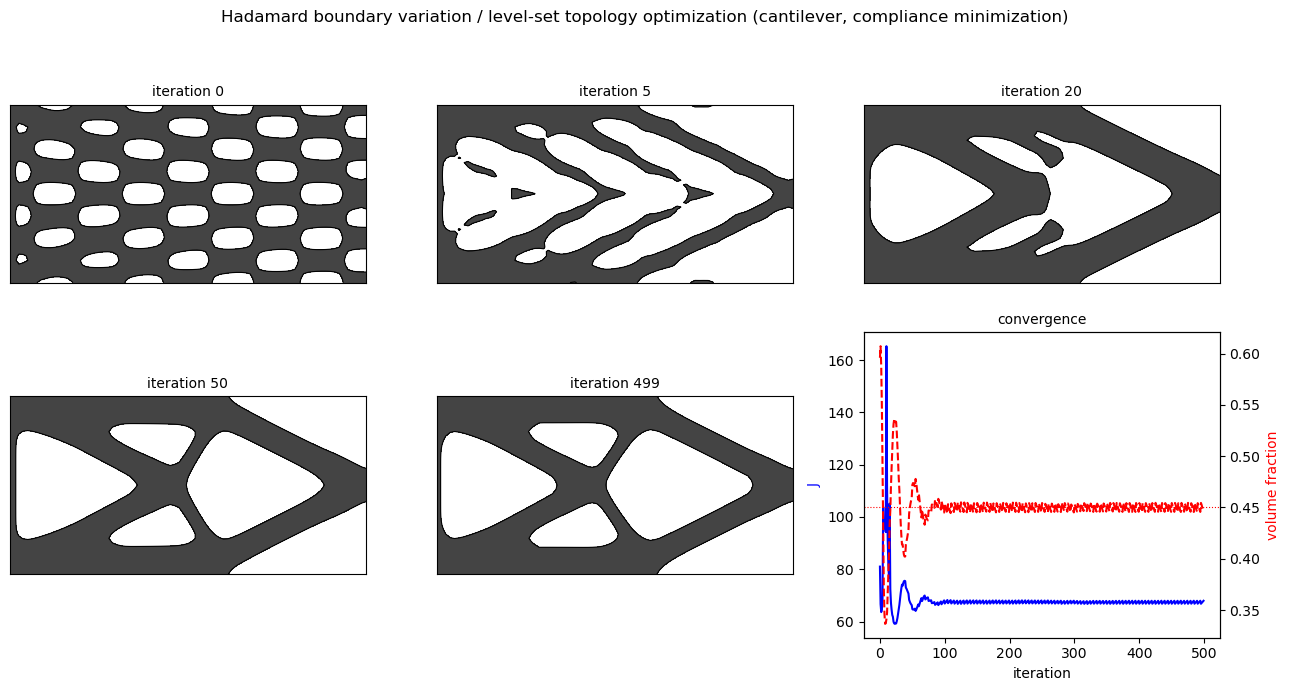
an augmented-Lagrangian / integral-control update: persistent volume excess steadily raises the price of material until the constraint is met. Like any integral controller it can overshoot, and the convergence plot shows exactly that - a damped oscillation of the volume around 0.45 that dies out over ~80 iterations. The penalty \(\mu\) is the control gain: too small and the volume drifts for dozens of iterations; too large and the oscillation amplifies. The mean-energy normalization of step 6 is what makes a single value (\(\mu = 2\)) work robustly.
10. Iteration step
Each iteration is four lines of structure:
rho, frac = density(phi)          # level set -> ersatz densities
U   = solve_elasticity(rho)       # state equation
v   = energy_to_nodes(U) - ell    # Hadamard shape gradient, extended to D
phi = reinitialize(advect(phi, v / |v|max, 8))   # HJ descent step
Starting from a plate perforated by ~40 seeded holes, the energy-driven velocity quickly eats the underloaded material; holes merge, thin members pinch off, and by iteration ~500 the design has collapsed to the canonical cantilever answer (see figure below): two chords running from the clamped edge to the load point, braced by an interior web - a continuum version of a two-bar truss. Compliance drops from its initial value and settles near \(J \approx 75\) with the volume locked at the target. None of those topology changes were “decided” anywhere in the code; they fall out of the level-set transport for free.
The full python script to generate this plot is provided at the end of this note.
11. Limitations
This code is for the tutorial purpose only, and it cuts the corners that production implementations do not. The velocity field is the raw energy density with no smoothing; a Helmholtz-type regularization (identifying the gradient in an \(H^1\) inner product instead of \(L^2\)) gives smoother boundaries and better mesh-independence. The descent has no line search or acceptance test, so the objective is not monotone. Hole nucleation is absent - the result can depend on the initial seeding - and the topological derivative would fix that. The point load is a singularity handled by crude clipping. And first-order upwinding smears the interface; WENO schemes and narrow-band solvers are the standard upgrades. None of these change the conceptual core: solve the PDE, read the shape gradient off the boundary, transport the level set, repeat.
References
- G. Allaire, F. Jouve, A.-M. Toader, Structural optimization using sensitivity analysis and a level-set method, J. Comput. Phys. 194 (2004) 363-393.
- M.Y. Wang, X. Wang, D. Guo, A level set method for structural topology optimization, Comput. Methods Appl. Mech. Engrg. 192 (2003) 227-246.
- S. Osher, J.A. Sethian, Fronts propagating with curvature-dependent speed, J. Comput. Phys. 79 (1988) 12-49.
- J. Céa, Conception optimale ou identification de formes: calcul rapide de la dérivée directionnelle de la fonction coût, RAIRO Modél. Math. Anal. Numér. 20 (1986) 371-402.
- G. Allaire, Conception optimale de structures, Springer, 2007 - the standard textbook treatment of Hadamard’s method.
Full python implementation
"""
Hadamard's boundary variation method for shape/topology optimization
===============================================================================
a minimal but mathematically faithful tutorial (NumPy/SciPy only).

THE IDEA IN 5 STEPS
-------------------
we minimize the compliance (work of the load = "softness") of an elastic
structure Omega inside a box D, under a volume constraint:

    min_{Omega in D}   J(Omega) = int_{Gamma_N} g . u ds
    s.t.               |Omega| = V_target,
    where u solves linear elasticity on Omega.

(1) HADAMARD'S BOUNDARY VARIATION.
    perturb the shape by a smooth vector field theta:
        Omega_theta = (Id + theta)(Omega).
    J is "shape differentiable" if  J(Omega_theta) = J(Omega) + dJ(Omega)(theta)
    + o(theta), with dJ linear in theta. Hadamard's structure theorem says the
    derivative only sees the NORMAL displacement of the boundary:
        dJ(Omega)(theta) = int_{Gamma} v * (theta . n) ds
    for some scalar field v on Gamma ("the shape gradient").

(2) THE SHAPE DERIVATIVE OF COMPLIANCE.
    for compliance, with the optimized boundary traction-free, a classical
    adjoint computation (the problem is self-adjoint) gives
        dJ(Omega)(theta) = - int_{Gamma} (A e(u) : e(u)) (theta . n) ds,
    where A e(u):e(u) is twice the elastic energy density. adding the volume
    constraint through a Lagrange multiplier ell, the Lagrangian
    L = J + ell |Omega| has
        dL(Omega)(theta) = int_{Gamma} (ell - A e(u):e(u)) (theta . n) ds.

(3) STEEPEST DESCENT = NORMAL VELOCITY.
    choosing theta . n = v_n with
        v_n = A e(u):e(u) - ell
    makes dL = -int v_n^2 < 0: a descent direction. physically: GROW the
    boundary where the material works hard (high energy density), SHRINK it
    where material is cheap to remove (energy below the "price" ell).

(4) LEVEL-SET TRANSPORT (Allaire-Jouve-Toader / Osher-Sethian).
    represent Omega = {phi < 0}. moving the boundary with normal speed v_n
    is exactly the Hamilton-Jacobi equation
        d(phi)/dt + v_n |grad phi| = 0,
    solved with an upwind (Godunov) scheme. this is what allows topology
    changes (holes merging/disappearing) while each instant is still a pure
    Hadamard boundary motion.

(5) ERSATZ MATERIAL.
    to avoid remeshing, the void D \\ Omega is filled with a very soft
    material (factor eps_void). the elasticity problem is always solved on
    the full box D with a Q4 (4-node bilinear quadrilateral) finite element mesh.

reference: G. Allaire, F. Jouve, A.-M. Toader, "structural optimization using
sensitivity analysis and a level-set method", J. Comput. Phys. 194 (2004).
"""

import numpy as np
import scipy.sparse as sp
import scipy.sparse.linalg as spla
import matplotlib.pyplot as plt

# ============================================================================
# parameters
# ============================================================================
nelx, nely = 80, 40   # elements in x, y  (box D = [0,80]x[0,40], h=1)
h          = 1.0      # mesh size
nu         = 0.3      # Poisson ratio (E = 1)
eps_void   = 1e-3     # ersatz material stiffness in the void
vol_target = 0.45     # target volume fraction |Omega| / |D|
n_iter     = 500      # optimization iterations
n_advect   = 8        # HJ time steps per iteration (pseudo-time)
reinit_every = 5      # reinitialize phi to a signed distance function
lag, mu    = 0.5, 2.0 # augmented Lagrangian: multiplier + penalty

# ============================================================================
# finite elements: Q4 stiffness matrix, mesh connectivity (plane stress)
# (classical "88-line" layout: node n = (nely+1)*ix + iy, y pointing down)
# ============================================================================
def lk(nu):
    k = np.array([1/2 - nu/6, 1/8 + nu/8, -1/4 - nu/12, -1/8 + 3*nu/8,
                  -1/4 + nu/12, -1/8 - nu/8, nu/6, 1/8 - 3*nu/8])
    return 1.0/(1 - nu**2) * np.array(
        [[k[0], k[1], k[2], k[3], k[4], k[5], k[6], k[7]],
         [k[1], k[0], k[7], k[6], k[5], k[4], k[3], k[2]],
         [k[2], k[7], k[0], k[5], k[6], k[3], k[4], k[1]],
         [k[3], k[6], k[5], k[0], k[7], k[2], k[1], k[4]],
         [k[4], k[5], k[6], k[7], k[0], k[1], k[2], k[3]],
         [k[5], k[4], k[3], k[2], k[1], k[0], k[7], k[6]],
         [k[6], k[3], k[4], k[1], k[2], k[7], k[0], k[5]],
         [k[7], k[2], k[1], k[4], k[3], k[6], k[5], k[0]]])

KE   = lk(nu)
ndof = 2 * (nelx + 1) * (nely + 1)
elx, ely = np.meshgrid(np.arange(nelx), np.arange(nely), indexing="ij")
n1 = ((nely + 1) * elx + ely).ravel()       # upper-left node of element
n2 = ((nely + 1) * (elx + 1) + ely).ravel() # upper-right node
edofMat = np.column_stack([2*n1+2, 2*n1+3, 2*n2+2, 2*n2+3,
                           2*n2,   2*n2+1, 2*n1,   2*n1+1])
iK = np.kron(edofMat, np.ones((1, 8), dtype=int)).ravel()
jK = np.kron(edofMat, np.ones((8, 1), dtype=int)).ravel()

# boundary conditions: cantilever. left edge clamped, unit downward point
# load at the middle of the right edge (this is Gamma_N; it is NOT optimized).
fixed = np.arange(2 * (nely + 1)) # all dofs at ix = 0
free  = np.setdiff1d(np.arange(ndof), fixed)
F = np.zeros(ndof)
load_node = (nely + 1) * nelx + nely // 2
F[2 * load_node + 1] = -1.0

def solve_elasticity(rho):
    """FEM solve on the whole box D with element-wise stiffness factor rho."""
    sK = (KE.ravel()[None, :] * rho.ravel()[:, None]).ravel()
    K  = sp.coo_matrix((sK, (iK, jK)), shape=(ndof, ndof)).tocsc()
    U  = np.zeros(ndof)
    U[free] = spla.spsolve(K[free][:, free], F[free])
    return U

# ============================================================================
# level set machinery. phi is defined on nodes, shape (nelx+1, nely+1).
# material Omega = {phi < 0}.
# ============================================================================
def upwind_diffs(p):
    """one-sided differences with edge replication (Neumann-like)."""
    q = np.pad(p, 1, mode="edge")
    Dxm = (p - q[:-2, 1:-1]) / h     # backward in x
    Dxp = (q[2:, 1:-1] - p) / h      # forward  in x
    Dym = (p - q[1:-1, :-2]) / h
    Dyp = (q[1:-1, 2:] - p) / h
    return Dxm, Dxp, Dym, Dyp

def godunov_norms(p):
    Dxm, Dxp, Dym, Dyp = upwind_diffs(p)
    gp = np.sqrt(np.maximum(Dxm, 0)**2 + np.minimum(Dxp, 0)**2 +
                 np.maximum(Dym, 0)**2 + np.minimum(Dyp, 0)**2)
    gm = np.sqrt(np.minimum(Dxm, 0)**2 + np.maximum(Dxp, 0)**2 +
                 np.minimum(Dym, 0)**2 + np.maximum(Dyp, 0)**2)
    return gp, gm

def advect(phi, v, steps):
    """Hamilton-Jacobi transport  phi_t + v |grad phi| = 0  (Godunov upwind).

    this is the discrete counterpart of Hadamard's boundary motion: the zero
    level set moves with normal velocity v (n = grad phi / |grad phi| points
    out of Omega since phi < 0 inside).
    """
    dt = 0.5 * h / max(np.abs(v).max(), 1e-12) # CFL condition
    for _ in range(steps):
        gp, gm = godunov_norms(phi)
        phi = phi - dt * (np.maximum(v, 0) * gp + np.minimum(v, 0) * gm)
    return phi

def reinitialize(phi, iters=40):
    """restore |grad phi| = 1 (signed distance) without moving {phi = 0},
    by integrating  phi_t + sign(phi)(|grad phi| - 1) = 0  to steady state.
    keeps the advection well-conditioned (level sets neither flatten nor
    bunch up)."""
    s = phi / np.sqrt(phi**2 + h**2)
    for _ in range(iters):
        gp, gm = godunov_norms(phi)
        g = np.where(s > 0, gp, gm)
        phi = phi - 0.5 * h * s * (g - 1.0)
    return phi

def density(phi):
    """element-wise material fraction from nodal phi (smeared interface),
    then ersatz interpolation rho in [eps_void, 1]."""
    eps = 1.5 * h                                  # smearing half-width
    chi = np.clip(0.5 - phi / (2 * eps), 0.0, 1.0) # ~ Heaviside(-phi)
    # average the 4 corner values of each element
    frac = 0.25 * (chi[:-1, :-1] + chi[1:, :-1] + chi[:-1, 1:] + chi[1:, 1:])
    return eps_void + (1 - eps_void) * frac, frac

# initial shape: material everywhere except a periodic array of holes
# (the level-set method can remove/merge holes but not nucleate them in 2D,
# so we seed the topology by hand as in Allaire et al.)
X, Y = np.meshgrid(np.arange(nelx + 1), np.arange(nely + 1), indexing="ij")
phi = -np.cos(8 * np.pi * X / nelx) * np.cos(8 * np.pi * Y / nely) - 0.1
phi = reinitialize(phi, 60)

def protect(phi):
    """keep a little material around the load point and the clamped edge so
    the load always has something to pull on."""
    r2 = (X - nelx)**2 + (Y - nely // 2)**2
    phi = np.where(r2 <= 9.0, np.minimum(phi, -0.5), phi)
    phi[0:2, :] = np.minimum(phi[0:2, :], -0.5)
    return phi

phi = protect(phi)

# ============================================================================
# optimization loop:  solve -> shape gradient -> advect -> reinitialize
# ============================================================================
history, snapshots = [], {}
snap_at = {0, 5, 20, 50, n_iter - 1}

for it in range(n_iter):
    rho, frac = density(phi)
    U = solve_elasticity(rho)
    J = F @ U # compliance
    vol = frac.mean() # volume fraction
    history.append((J, vol))

    # element energy density  A e(u):e(u)  (with ersatz factor), -> nodes
    Ue = U[edofMat]
    ee = rho.ravel() * np.einsum("ij,jk,ik->i", Ue, KE, Ue)
    ee_el = ee.reshape(nelx, nely)
    ee_nd = np.zeros((nelx + 1, nely + 1))
    cnt   = np.zeros((nelx + 1, nely + 1))
    for dx in (0, 1):
        for dy in (0, 1):
            ee_nd[dx:nelx+dx, dy:nely+dy] += ee_el
            cnt[dx:nelx+dx, dy:nely+dy] += 1
    ee_nd /= cnt
    # clip the load-point singularity so it does not dominate the velocity,
    # and normalize by the mean energy so the multiplier ell is O(1)
    ee_nd = np.minimum(ee_nd, np.quantile(ee_nd, 0.999))
    ee_nd = ee_nd / max(ee_nd.mean(), 1e-12)

    # augmented-Lagrangian multiplier for the volume constraint
    ell = lag + mu * (vol - vol_target)
    lag = ell

    # Hadamard steepest descent: normal velocity v_n = A e(u):e(u) - ell.
    # (>0 grows Omega, <0 shrinks it; see header, steps (2)-(3).)
    v = ee_nd - ell
    v = v / max(np.abs(v).max(), 1e-12) # normalize speed

    phi = advect(phi, v, n_advect)
    phi = protect(phi)
    if (it + 1) % reinit_every == 0:
        phi = reinitialize(phi)

    if it in snap_at:
        snapshots[it] = phi.copy()
    if it % 10 == 0 or it == n_iter - 1:
        print(f"iter {it:3d}   J = {J:7.3f}   vol = {vol:.3f}   ell = {ell:5.3f}")

# ============================================================================
# plots
# ============================================================================
hist = np.array(history)
fig = plt.figure(figsize=(13, 7))
for k, it in enumerate(sorted(snapshots)):
    ax = fig.add_subplot(2, 3, k + 1)
    ax.contourf(snapshots[it].T, levels=[-1e9, 0], colors=["#444444"])
    ax.contour(snapshots[it].T, levels=[0], colors="k", linewidths=0.8)
    ax.set_title(f"iteration {it}", fontsize=10)
    ax.set_aspect("equal"); ax.invert_yaxis(); ax.set_xticks([]); ax.set_yticks([])

ax = fig.add_subplot(2, 3, 6)
ax.plot(hist[:, 0], "b-", label="compliance J")
ax.set_xlabel("iteration"); ax.set_ylabel("J", color="b")
ax2 = ax.twinx()
ax2.plot(hist[:, 1], "r--", label="volume")
ax2.axhline(vol_target, color="r", ls=":", lw=0.8)
ax2.set_ylabel("volume fraction", color="r")
ax.set_title("convergence", fontsize=10)

fig.suptitle("Hadamard boundary variation / level-set topology optimization "
             "(cantilever, compliance minimization)", fontsize=12)
fig.tight_layout()
plt.show()